Observations of the Atlantic Meridional Overturning Circulation (AMOC)
The Atlantic Meridional Overturning Circulation (AMOC) is comprised of a series of northward surface currents and southward currents at depth in the Atlantic Basin. It is a key part of the global ocean circulation and is responsible for substantial oceanic heat transport, deep water formation, and controlling regional climate. It is possible that climate change has and will continue to affect the strength of AMOC and observations of this system are critical for validating model experiments of the circulation. Multiple observing systems across the Atlantic basic work together to measure the AMOC. There is no one single observing system, nor is there a one-stop shop for data access. Users need to decide which dataset to use based on their specific interests. The following observing systems typically express AMOC as the volume of seawater transported across a line as part of AMOC. These volume transports are calculated as the sums of multiple components such as currents at the boundary, in the interior, and wind-driven currents near the surface. For comparisons with output from numerical models, it may be appropriate to compare the resulting AMOC directly, to reproduce the calculation methods in the model output, or to compare the underlying in-situ data such as temperature, salinity, or boundary current speeds. In addition to observing systems that attempt to capture the whole AMOC, this page also includes observing systems that capture important sub-components of the circulation, such as boundary currents in specific locations.
Key Strengths
Observational records are now several decades long, making them long enough to address decadal variability
Some of the records provide well-calibrated data from the deep ocean where data availability is generally very low
Key Limitations
There is no one AMOC data set. Instead, there are multiple independent projects, which each use different methodology to derive AMOC from their specific observational setup.
Users have to figure out which data set(s) may be best to use for their particular use case or science question and how the methodology and the underlying assumptions affect the outcome.
Expert User Guidance
The following was contributed by Matthias Lankhorst, Scripps Institution of Oceanography, July 2025:
Introduction
The Atlantic Meridional Overturning Circulation (AMOC) is the large-scale system of currents in the Atlantic Ocean that transports warm water northward in the upper water column, and colder water southward at depth. It plays an important role in the climate system due to its heat transport (e.g., Trenberth and Fasullo, 2017), and the Atlantic is special in that heat is transported northward in both hemispheres (as opposed to poleward). Knowledge of e.g. the Gulf Stream and that its temperature is higher than surrounding waters dates back many years, and has been documented in early navigational charts such as those by B. Franklin (cf. Richardson, 1980). Bower et al. (2019) review the pathways of AMOC throughout the entire Atlantic, both of the upper and lower limbs, and show a number of recirculations and eddies to make clear that AMOC is more than a simple, north-south laminar flow through the ocean.
There is no single observing system that describes the AMOC. Instead, there are a number of individual projects that make dedicated observations at different locations, each using different methods and assumptions. These projects typically include observations from moorings as their primary source of in-situ data. A selection of projects is outlined here, including an overview of methods and links to data repositories, followed by some additional remarks about the peculiarities of mooring-based oceanographic data. In addition to individual observational projects dedicated to AMOC, there are analyses that derive AMOC-relevant metrics from other, more general observational datasets such as satellite altimetry and Argo float data. A small selection of such analyses is presented here as well.
The strength of the AMOC is usually provided as a volume transport in units of Sverdrup (1 Sv = 106 m3/s), and denotes the volume of seawater that flows across a section over time. “Overturning” is generally understood such that this volume of water flows in one direction in the upper ocean, and this is compensated by an equal but opposite flow at depth. Variations of this understanding exist between the different observing systems (cf. below): E.g., RAPID generally follows this concept, MOVE only observes one of the two layers (the deep one), and OSNAP replaces the concept of overturning in the vertical by one that happens in density coordinates, with the actual flow patterns being more horizontally separated.
Users of AMOC observations will have to decide whether they want to use a measure of AMOC itself, or whether use of the underlying observations such as temperature, salinity, and currents at select locations is more appropriate. This is particularly true when comparing observational data to those from numerical models. The observational AMOC results critically depend on small density gradients between very specific water masses in very specific locations and depths, as well as narrow and swift current pathways along the basin boundaries. These processes are notoriously difficult to reproduce with fidelity in models. Therefore, the details in the model world might be different from those in reality, and a true apples-to-apples comparison may be elusive. Danabasoglu et al. (2021) provide an example of comparing numerical model simulations with AMOC observations, and highlight some of these issues by reproducing the observational methods in the model data.
Ongoing AMOC Observing Systems
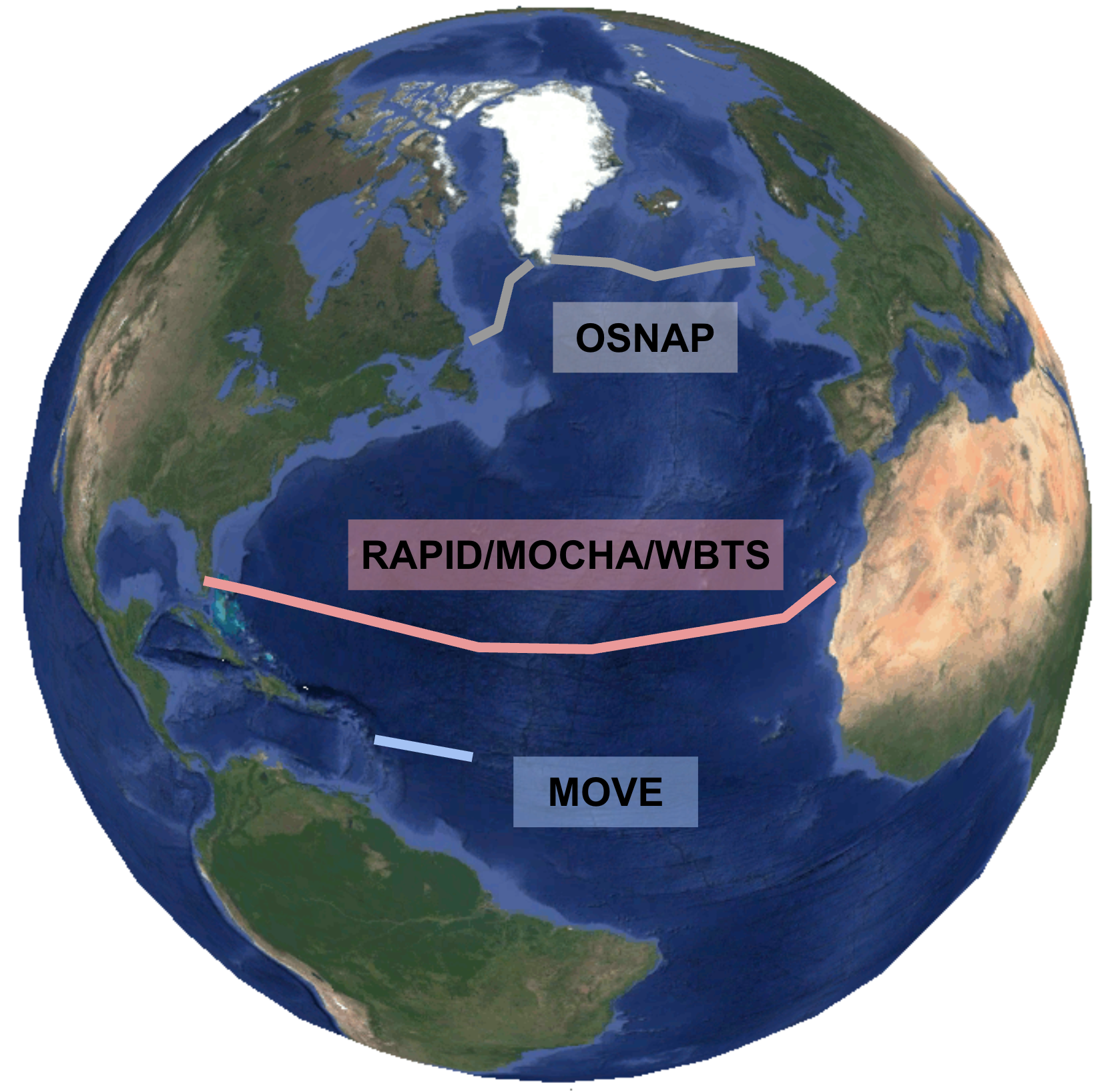
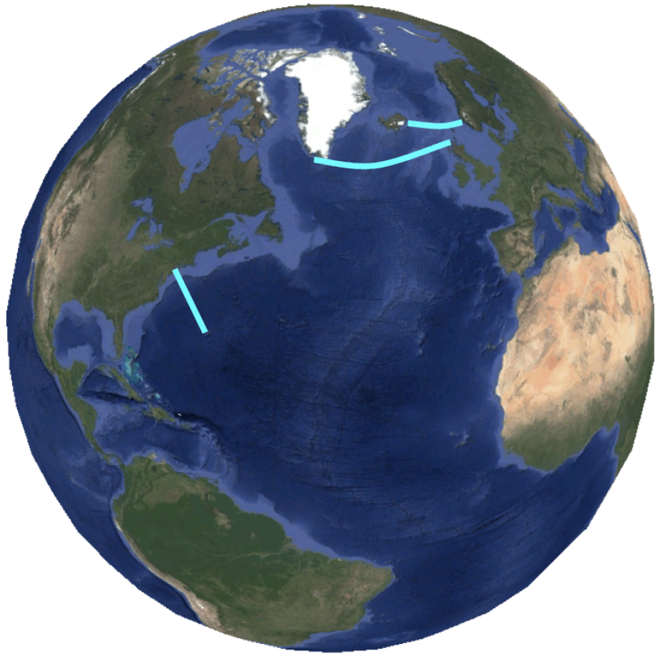
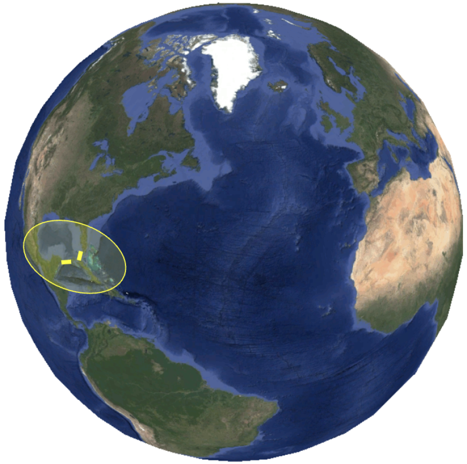
An overview of continuous AMOC observations from dedicated arrays was given by Frajka-Williams et al. (2019), and is still reasonably up-to-date (as of 2025). The locations of these arrays are shown in the figure below and the following summary tables introduce each array. For more detailed information about each array, readers are referred to Frajka-Williams et al. (2019) as well as the websites and publications listed here in the summary tables.
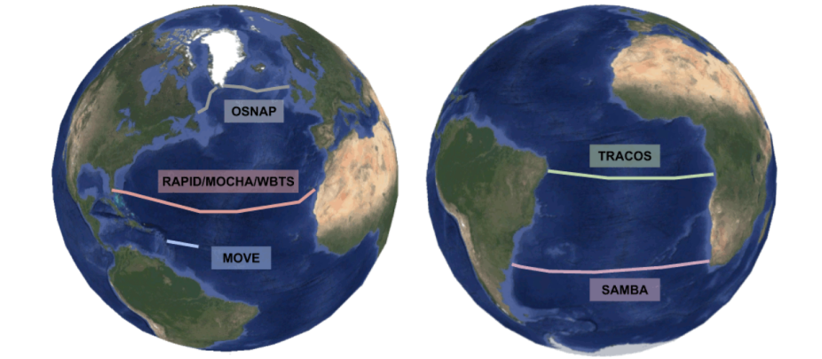
Maps of ongoing AMOC observing array locations in the North and South Atlantic (left and right panels, resp.). Note that the positions are approximate.
Matthias Lankhorst
| OSNAP – Overturning in the Subpolar North Atlantic Program | |
| Description | OSNAP makes observations of AMOC across a line that stretches from Labrador to Greenland, and onwards to Scotland. The observing system consists of multiple mooring arrays in key locations on this line, plus a section in the east that is covered with gliders. Some of the observations are from direct current meters, while for other parts of the section, geostrophic flow is calculated from density (temperature and salinity) observations. Surface altimetry observations are used to determine the reference velocity for the geostrophic flow. In addition, an assumption of net-zero flow across the section is made and implemented through compensation flows that are partitioned among the western and eastern parts of the OSNAP line. AMOC metrics from OSNAP are calculated from the overturning as seen in density coordinates, which is different from depth coordinates in this location. |
| Website | https://www.o-snap.org/ |
| Select Publications | Fu et al. (2023) Lozier et al. (2019) |
| Data Access | https://www.o-snap.org/data-access/ https://doi.org/10.35090/gatech/70342 |
| RAPID/MOCHA/WBTS (26°N) | |
| Description | A merger of three separate projects (Rapid Climate Change, Meridional Overturning Circulation and Heat-flux Array, Western Boundary Time Series), this array makes AMOC observations in the subtropical North Atlantic where the AMOC heat transport is near its maximum. The observing system combines data from the Florida Straits cable observations, open-ocean mooring data that in turn are a combination of direct current meters and density (temperature, salinity) observations, and wind-driven near-surface current estimates. The reference level for the geostrophic flow from density observations is derived via an assumption of net-zero flow across the array, and implemented through a compensation term of a particular shape. Websites below link to AMOC data as well as individual mooring and cable data. |
| Website | https://rapid.ac.uk/ |
| Select Publications | McCarthy et al. (2015) Smeed et al. (2018) |
| Data Access | https://rapid.ac.uk/data https://www.aoml.noaa.gov/phod/wbts/data.php |
| MOVE – Meridional Overturning Variability Experiment (16°N) | |
| Description | MOVE makes mooring-based observations of the deep branch of AMOC at a location in the tropical Atlantic. At this location, the flow is confined by the topography such that the observations can be made with a comparatively small amount of instrumentation. The flow is calculated as the sum of a component directly at the boundary that is observed with current meters, an internal component that is derived from density (temperature, salinity) observations and geostrophy, and an external component that provides the reference level for the geostrophy from seafloor pressure observations. On long time scales, the reference level is assumed as constant flow at depth. Numerical simulations have shown that the deep flow derived via this method represents the total AMOC well on time scales of multiple years and longer. |
| Website | https://mooring.ucsd.edu/move/ |
| Select Publications | Kanzow et al. (2006) Send et al. (2011) |
| Data Access | Access through NOAA OceanSITES ftp://ftp.ifremer.fr/ifremer/oceansites/DATA/ (folders MOVE*) |
| TRACOS – Tropical Atlantic Circulation and Overturning at 11°S | |
| Description | TRACOS makes observations of seafloor pressure, as well as mooring-based observations of currents and density (temperature, salinity), off the coasts of South America and Africa in the tropical South Atlantic. Combined with satellite altimetry data and estimates of wind-driven flow, these allow for an estimate of AMOC flow variability across this section. Details of the methodology and data dissemination are still work in progress (as of 2025). |
| Website | https://www.geomar.de/en/fb1/physical-oceanography/long-term-observations/tracos-11s |
| Select Publications | Hummels et al. (2015) Herrford et al. (2021) |
| Data Access | (available upon request to PIs) |
| SAMBA – South Atlantic MOC Basin-Wide Array (34.5°S) | |
| Description | SAMBA is a merger of several components that make observations of seafloor pressure, as well as mooring-based observations of currents and density (temperature, salinity), off the coasts of South America and Africa near the latitude of the southern tip of Africa, as well as in the open ocean. Together, these form a trans-basin array and allow for an estimate of AMOC flow across this section. Detailed publication of the methodology and complete data dissemination are still work in progress (as of 2025). |
| Websites | https://www.aoml.noaa.gov/phod/SAMOC_international/index.php https://www.aoml.noaa.gov/sam/ |
| Select Publications | Meinen et al. (2018) |
| Data Access | Partial access through NOAA AOML, contact PIs for additional raw instrumental data |
Other Relevant Observing Systems and Studies
There are numerous other observational studies that examine components of AMOC, either ongoing or concluded. The following list is a selection of such studies, likely incomplete and not doing justice to those not listed. This is provided here to provide pointers to additional data sources for users that are interested in more details.
| Greenland-Iceland-Scotland Ridge | |
|
|
Multiple observational records exist for the throughflow over the shallow passages between Greenland, Iceland, the Faroe Islands, and Scotland. These cover select parts of the cold deep southward overflows, as well as the warm near-surface poleward currents. The list below is likely incomplete, but a good starting point to identify available records and publications. |
| Website | (n/a) |
| Hansen et al. (2023) Larsen et al. (2024) Mayer et al. (2023) Jochumsen et al. (2017) |
|
| https://envofar.fo/index.php?page=climate https://envofar.fo/data/index.php?dir=Timeseries&sort=N&order=A https://www.cen.uni-hamburg.de/en/icdc/data/ocean/denmark-strait-overflow.htm |
|
| Indices of the Subpolar Gyre, North Atlantic Current, AMOC at 41°N, and the OVIDE Line | |
|
|
This is a selection of indices derived from altimetry observations, and combinations of these with Argo and other in-situ data. Häkkinen and Rhines (2004) show an index that describes the strength of the subpolar gyre (SPG). Lankhorst and Send (2020) calculate the flow in the North Atlantic Current (NAC) and provide uncertainty estimates. Willis (2010) derives an index that represents the AMOC at 41°N. OVIDE (Observatoire de la variabilité interannuelle et décennale en Atlantique Nord) makes measurements to assess the flow across a line from Greenland to Portugal. |
| Website | (none for SPG, NAC, 41°N) https://www.umr-lops.fr/en/Projects/Active-projects/OVIDE |
| Häkkinen and Rhines (2004); Berx and Payne (2017) – SPG Lankhorst and Send (2020) – NAC Willis (2010); Hobbs and Willis (2012) – 41°N Mercier et al. (2024) – OVIDE |
|
| https://doi.org/10.7489/1806-1 (SPG) https://doi.org/10.6075/J00Z747J (NAC) https://doi.org/10.5281/zenodo.8170365 (41°N) https://www.umr-lops.fr/en/Projects/Active-projects/OVIDE/Ovide-data (OVIDE) |
|
| NOAC – North Atlantic Changes (47°N) | |
|
|
NOAC is an array that spans the North Atlantic between the Grand Banks and the British Isles, and makes observations from seafloor instruments and a small number of moorings. These are used to construct an AMOC time series together with a wind-driven component, extrapolations beyond the array boundaries from external datasets, and an assumption of net-zero mass balance to determine the reference level for geostrophic velocities. |
| Website | (n/a) |
| Wett et al. (2023) | |
| https://doi.org/10.1594/PANGAEA.959558 https://doi.org/10.1594/PANGAEA.925089 https://doi.org/10.1594/PANGAEA.903211 |
|

| Line W and RAPID WAVE | |
|
|
RAPID West Atlantic Variability Experiment (WAVE) equipped two sections on the continental slope with seafloor instruments, and Line W was a mooring array across the slope, all at locations off eastern North America. Data show the Deep Western Boundary Current along the shelf, and surface flow inshore of, and reaching partially out to, the Gulf Stream. |
| Website | https://scienceweb.whoi.edu/linew/index.php https://www.bodc.ac.uk/data/documents/nodb/78116/ |
| Toole et al. (2011) Elipot et al. (2013) |
|
| https://hdl.handle.net/1912/28660 (Line W) https://www.bodc.ac.uk/data/bodc_database/nodb/search/ (use search function by project, “RAPID-WAVE”, and platform, “fixed benthic node”) |
|

| Volunteer Observing Ships Norröna, Nuka Arctica, and Oleander | |
|
|
Three volunteer observing ship (VOS) projects are highlighted here because they were equipped with ADCP instruments that directly observe key AMOC current features: Norröna covers a section from Iceland to mainland Europe that spans the North Atlantic Current inflow into the Nordic Seas, Nuka Arctica covers the North Atlantic and Irminger Currents a bit further south between Greenland and mainland Europe, and Oleander covers the Gulf Stream between mainland North America and Bermuda. |
| Website | http://po.msrc.sunysb.edu/Norrona/ https://bios.asu.edu/oleander |
| Childers et al. (2015) – Norröna and Nuka Arctica Rossby et al. (2019) – Oleander |
|
| https://uhslc.soest.hawaii.edu/sadcp/INVNTORY/norrona.html http://po.msrc.sunysb.edu/Norrona/#Data http://erddap.oleander.bios.edu:8080/erddap/info/index.html |
|
| Canek – Yucatan Channel and Florida Straits Arrays to Observe the Loop Current | |
|
|
Canek refers to an array of current meter moorings in Yucatan Channel. There is a second array in the Florida Straits, and both together observe the Loop Current as it enters and leaves the Gulf of Mexico. |
| Website | (n/a) |
| Candela et al. (2019) | |
| https://doi.org/10.5281/zenodo.7865541 (Yucatan Channel only) | |
Mooring Data: “Gridded” versus “Native” Resolution, and Effects of Mooring Motion
While we tend to think of mooring-based observations as fixed in their locations, there are some nuances to this that matter for interpretation of the data. The mooring structures do move when exposed to ambient currents. In the case of a subsurface mooring, this usually means that the structure tilts sideways, and in doing so, instruments fixed on the mooring riser end up at depths greater than their nominal depths. For analysis purposes, this depth change usually matters more than the lateral displacement. The Figure below illustrates the point. Mooring observations might be published either at the native instrumental resolution, in which case the data from one instrument will likely be from different depths throughout its deployment, and/or in a version that is “gridded” on fixed vertical levels using some interpolation and averaging algorithm. Users of mooring data need to understand whether the data have been processed this way or not, else the interpretation will be very wrong (in the worst case in the figure below, one might wrongfully think that a temperature measurement from 700 m was from 30 m). Metadata in the mooring data files should make this clear.
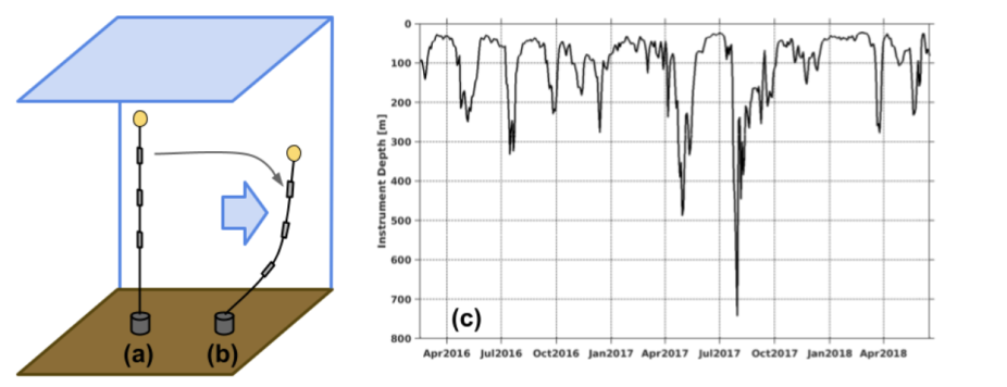
Example of mooring knockdown. In its nominal configuration (a), the mooring riser is held upright by flotation (yellow sphere), and instruments on the riser (grey boxes) are at their nominal depths. Ambient currents (blue arrow) can cause the mooring to tilt (b), and the instrument depths are now different from nominal (grey arrow). Panel (c) shows an actual depth record from an instrument that was nominally at 30 m depth on a MOVE mooring, but was displaced down (and sideways, not shown) by hundreds of meters on several occasions.
Matthias Lankhorst
Mooring Data: Miscellaneous Details and Pitfalls to Avoid
- When observational data are provided at the native instrumental resolution, there are two options how quality control addresses “bad” data: One is to remove bad data points (which could be actual deletion of data points or replacement with dummy values), the other is to leave all data points in but add quality control flags that show the quality of each data point. The latter is common, and guards against accidental loss of data by a quality control method that is too strict. A user needs to understand how this is dealt with in a given dataset. If there are quality flags, users need to know what they mean and how to filter out bad data themselves. This information is usually contained in the metadata.
- Users of mooring-based seawater temperature data need to understand if the data represent the in-situ temperature, potential temperature, or absolute temperature. This information is usually contained in the metadata. Note also that the temperature scale was redefined in 1990 – present-day observations are typically reported on this ITS-90 scale, but historical data may be based on earlier scale definitions, such as IPTS-68.
Users of mooring-based salinity data need to understand whether the data represent practical or absolute salinity. This information is usually contained in the metadata. - Users of mooring-based pressure data need to understand whether the atmospheric pressure has been subtracted or not (i.e. whether the instrument should read about zero or about ten dbar at the sea surface). For pressure data from seafloor landers, data processing often includes removal of means, trends, and/or tides, and a user of a given dataset needs to understand what stage of processing the data are at. This information is usually contained in the metadata.
- Oceanographic data files in NetCDF file format often follow the CF and ACDD metadata conventions. NetCDF files contain metadata fields, called attributes, that describe either individual data variables inside a file, or the content of the entire file. Many of the aforementioned questions about data details can be answered by reading the attributes “standard_name” (comes from a standardized list in CF) and “units” for a particular variable. These should uniquely define what physical quantity is contained in the variable, and in what physical units the data are given.
Mooring Data: Access at OceanSITES
OceanSITES (Send et al., 2010) is an international program to “collect, deliver and promote the use of high-quality data from long-term, high-frequency observations at fixed locations in the open ocean” (OceanSITES mission statement). The majority of these are mooring-based observations. For some, but not all, of the AMOC projects discussed here, OceanSITES is the umbrella organization, and their data are disseminated through the OceanSITES data portals. There are two such portals, referred to as GDACs (global data access center), which hold identical copies of the data. One GDAC is at the NOAA National Data Buoy Center (NDBC) in the US, the other at Ifremer in France. Each one offers several methods/protocols to access the data, which change over time as the technology evolves (initially ftp servers, then moving to additional and/or more secure services such as sftp or THREDDS). OceanSITES data are organized into two categories: at the original instrumental resolution organized by individual sites, and any higher-order processing such as gridding, merging multiple deployments into single files, or derived products. The data at the native resolution is provided in a top-level directory called “DATA”, and organized further by sites. Data files are usually per deployment, and data from separate instruments may be in separate files, which makes them harder to use. Data from higher-order processing are in a top-level directory called “DATA_GRIDDED”. All data files are in NetCDF format, and OceanSITES provides information about metadata content and formats via their website.
Mooring Data: Importance of Calibrations for Deep-Ocean Observations
Signals in the deep ocean are small, and possibly near the detection limits of the instrumentation. Yet, some of the AMOC calculations used by the observational arrays critically depend on these signals. Here, this typically concerns the density data used in the geostrophic flow calculations, and of the underlying CTD data, especially the conductivity is affected. Kanzow et al. (2006) document a method for additional mooring sensor calibration to address this, and Anderson et al. (2020) report certain issues that can still linger in data from abyssal depths after such calibrations. A user of observational AMOC data may not need to understand all the issues in great detail, but should at least have a general knowledge of their existence, and that residual sensor drift issues can degrade the resulting AMOC data.
Seafloor Pressure Data: Drift, Tides, Mean Flow
Several of the AMOC arrays use seafloor pressure observations to derive geostrophic flow directly from the observed pressure gradients between two sites. Such pressure data have a number of shortcomings:
- The mean value of a seafloor pressure record is usually not well-determined, for two reasons: Firstly, absolute sensor calibration is often not accurate to the small numbers needed (order of millimeters water equivalent), and the sensor placement in absolute earth coordinates is not known to this level of accuracy either (to calculate horizontal gradients, one would have to know that the two sensors are at the same level to such an accuracy). Therefore, the mean value of the resulting flow needs to be determined via some different method, such as an assumption of reference level or mass balance.
- Pressure sensors drift: Kanzow et al. (2006) show possible corrections for such drift from empirical fits of exponential-linear curves to the data, but these inherently remove long-term signals from the data along with the drift. Some independent assessments need to be made for the missing long-term signals and trends, possibly also via assumptions of reference level or mass balance.
- The biggest signals in pressure records tend to be tides. Even after applying standard filters to remove the tides, there may still be residuals that are large enough to interfere with the desired signals. Careful choices of filters are required for this purpose.
- In some locations, the seafloor is subject to tectonic motion, invalidating the assumption that the sensor is fixed in the vertical direction. Such situations are difficult to interpret without additional geophysical data, such as the occurrence of earthquakes.
More Questions
What are the key strengths of this data set?
Some of the observational records are now several decades long, which makes them long enough to address decadal variability. Also, some of the records provide well-calibrated data from the deep ocean, where data availability is generally very low.
What are the key limitations of this data set?
There is no one AMOC data set. Instead, there are multiple independent projects, which each use different methodology to derive AMOC from their specific observational setup.
What are the typical research applications of this data set?
To study whether AMOC is changing (on time scales over many years), and whether AMOC data from different locations are changing consistently (e.g. coherent changes over multiple latitudes).
What are the most common mistakes that users encounter when processing or interpreting these data?
- Ignoring the assumptions that went into the calculations of AMOC from the actual observed variables, and that they might impact the resulting AMOC signals. E.g. is a trend in the AMOC real, or an artefact of a reference level assumption?
- Assuming that numerical models reproduce the exact details of the topography (such as narrow passages or steep boundaries), and exact details of water masses and their motion (e.g. is the North Atlantic Deep Water at the corrected depths, does it have the same temperature-salinity properties as the observations, are the narrow boundary currents at the right locations and depths?).
What are some comparable data sets, if any?
Meridional heat transport is the primary reason we are interested in the AMOC. Some of the AMOC arrays actually provide estimates of this heat transport as well. There are AMOC metrics that are implied from other observations (e.g. changes in oceanic heat content that are not explained by air-sea fluxes locally can be inferred to be from AMOC).
How is uncertainty characterized in these data?
Several, but not all, of the AMOC arrays discuss how large their sensor uncertainties may be, and how that would propagate into AMOC uncertainty (e.g., Kanzow et al., 2006; Lankhorst and Send, 2020). However, comprehensive error analyses that take into account the sampling errors in addition to the sensor errors and reference level assumptions are very difficult to make. Users should carefully study the publications about a particular array to find more details.
Were corrections made to account for changes in observing systems or practices, sampling density, satellite drift, or similar issues?
Yes, most arrays use some combination of sensor drift correction, as discussed above for the deep-ocean data as well as seafloor pressure data.
How useful are these data for characterizing means as well as extremes?
In general, the resulting mean AMOC value from each observational array is dependent on some of the underlying assumptions (reference level, mass balance), i.e. possibly not a fully independent measurement. Variability around this mean, including extreme events, is generally observed with higher confidence.
How does one best compare these data with model output?
Carefully consider whether to compare the AMOC numbers, or the underlying in-situ variables such as temperature and salinity, or both. A basic understanding of how the model represents key water masses and currents involved in AMOC is necessary to avoid comparing “apples to oranges”: E.g. MOVE considers the deep flow in a specific depth range (approx. 1200-5000 m, carrying the North Atlantic Deep Water) and interprets this as a measure of AMOC. One should not use model output velocities from the same depth range blindly, but rather confirm that the model produces a water mass like North Atlantic Deep Water, and then perhaps use the (possibly different) depth range where this flows in the model. Danabasoglu et al. (2021) show examples of some of these comparisons.
Are there spurious (non-climatic) features in the temporal record?
Yes! Trend removal in seafloor pressure data removes certain low-frequency signals in some arrays, and assumptions of geostrophic reference levels impose their inaccuracy on the resulting AMOC numbers. The details vary between observing systems.
How do I access these data?
The tables above include links, which were current at the time of writing (mid-2025). If some datasets from these links are incomplete, inquiries to the authors are encouraged.
How frequently are the data updated?
Mooring-based arrays are typically updated every one to two years, which corresponds to the service intervals of the instrumentation.
Is there any publicly available code that illustrates how to access and analyze these data? If so, where?
A software package called METRIC, published by F. Castruccio, is available on Zenodo and GitHub to extract data from numerical model output fields and process them in a way similar to a select number of the observational arrays. Further details are provided by Danabasoglu et al. (2021). There is also an AMOC community site on GitHub, with basic software to read and plot data in a repository called amocarray. E. Frajka-Williams’s GitHub site contains additional code for some instruments and datasets.
References
Anderson, N.D., Donohue, K.A., Honda, M.C., Cronin, M.F. and Zhang, D., 2020. Challenges of measuring abyssal temperature and salinity at the Kuroshio extension observatory. Journal of Atmospheric and Oceanic Technology, 37(11), pp.1999-2014. https://doi.org/10.1175/JTECH-D-19-0153.1
Bower, A., Lozier, S., Biastoch, A., Drouin, K., Foukal, N., Furey, H., Lankhorst, M., Rühs, S. and Zou, S., 2019. Lagrangian views of the pathways of the Atlantic Meridional Overturning Circulation. Journal of Geophysical Research: Oceans, 124(8), pp.5313-5335. https://doi.org/10.1029/2019JC015014
Candela, J., Ochoa, J., Sheinbaum, J., Lopez, M., Perez-Brunius, P., Tenreiro, M., Pallàs-Sanz, E., Athié, G. and Arriaza-Oliveros, L., 2019. The flow through the Gulf of Mexico. Journal of Physical Oceanography, 49(6), pp.1381-1401. https://doi.org/10.1175/JPO-D-18-0189.1
Childers, K.H., Flagg, C.N., Rossby, T. and Schrum, C., 2015. Directly measured currents and estimated transport pathways of Atlantic water between 59.5° N and the Iceland–Faroes–Scotland Ridge. Tellus A: Dynamic Meteorology and Oceanography, 67(1), p.28067. https://doi.org/10.3402/tellusa.v67.28067
Danabasoglu, G., Castruccio, F.S., Small, R.J., Tomas, R., Frajka‐Williams, E. and Lankhorst, M., 2021. Revisiting AMOC transport estimates from observations and models. Geophysical Research Letters, 48(10), p.e2021GL093045. https://doi.org/10.1029/2021GL093045
Elipot, S., Hughes, C., Olhede, S. and Toole, J., 2013. Coherence of western boundary pressure at the RAPID WAVE array: Boundary wave adjustments or deep western boundary current advection?. Journal of physical oceanography, 43(4), pp.744-765. https://doi.org/10.1175/JPO-D-12-067.1
Fu, Y., Li, F., Johns, W.E., and Lozier, M.S., 2023. Calculation method summary. OSNAP technical report. Georgia Institute of Technology. https://doi.org/10.35090/gatech/72190
Jochumsen, K., Moritz, M., Nunes, N., Quadfasel, D., Larsen, K.M.H., Hansen, B., Valdimarsson, H., and Jonsson, S., 2017. Revised transport estimates of the Denmark Strait overflow, J. Geophys. Res. Oceans, 122, 3434–3450, https:/doi.org/10.1002/2017JC012803
Häkkinen, S. and Rhines, P.B., 2004. Decline of subpolar North Atlantic circulation during the 1990s. Science, 304(5670), pp.555-559. https://doi.org/10.1126/science.1094917
Hansen, B., Larsen, K. M. H., Hátún, H., Olsen, S. M., Gierisch, A. M. U., Østerhus, S., and Ólafsdóttir, S. R., 2023. The Iceland-Faroe warm-water flow towards the Arctic estimated from satellite altimetry and in situ observations, Ocean Sci., 19, 1225-1252. https://doi.org/10.5194/os-19-1225-2023
Herrford, J., Brandt, P., Kanzow, T., Hummels, R., Araujo, M. and Durgadoo, J.V., 2021. Seasonal variability of the Atlantic Meridional Overturning Circulation at 11°S inferred from bottom pressure measurements. Ocean Sci., 17, 265–284. https://doi.org/10.5194/os-17-265-2021
Hobbs, W. R., and J. K. Willis, 2012. Midlatitude North Atlantic heat transport: A time series based on satellite and drifter data. J. Geophys. Res., 117, C01008, https://doi.org/10.1029/2011JC007039
Hummels, R., Brandt, P., Dengler, M., Fischer, J., Araujo, M., Veleda, D., and Durgadoo, J.V., 2015. Interannual to decadal changes in the western boundary circulation in the Atlantic at 11°S, Geophys. Res. Lett., 42, 7615–7622, https://doi.org/10.1002/2015GL065254
Kanzow, T., Send, U., Zenk, W., Chave, A.D. and Rhein, M., 2006. Monitoring the integrated deep meridional flow in the tropical North Atlantic: Long-term performance of a geostrophic array. Deep Sea Research Part I: Oceanographic Research Papers, 53(3), pp.528-546. https://doi.org/10.1016/j.dsr.2005.12.007
Lankhorst, M. and Send, U., 2020. Uncertainty of North Atlantic Current observations from altimetry, floats, moorings, and XBT. Progress in Oceanography, 187, p.102402. https://doi.org/10.1016/j.pocean.2020.102402
Larsen, K. M. H., Hansen, B., Hátún, H., Johansen, G. E., Østerhus, S., and Olsen, S. M., 2024. The Coldest and Densest Overflow Branch into the North Atlantic is Stable in Transport, but Warming. Geophysical Research Letters, 51, e2024GL110097. https://doi.org/10.1029/2024GL110097
Lozier, M.S., Li, F., Bacon, S., Bahr, F., Bower, A.S., Cunningham, S.A., de Jong, M.F., de Steur, L., deYoung, B., Fischer, J. and Gary, S.F., 2019. A sea change in our view of overturning in the subpolar North Atlantic. Science, 363(6426), pp.516-521. https://www.doi.org/10.1126/science.aau6592
Mayer, M., Tsubouchi, T., Winkelbauer, S., Larsen, K. M. H., Berx, B., Macrander, A., Iovino, D., Jónsson, S., and Renshaw, R., 2023. Recent variations in oceanic transports across the Greenland–Scotland Ridge, in: 7th edition of the Copernicus Ocean State Report (OSR7), edited by: von Schuckmann, K., Moreira, L., Le Traon, P.-Y., Grégoire, M., Marcos, M., Staneva, J., Brasseur, P., Garric, G., Lionello, P., Karstensen, J., and Neukermans, G. Copernicus Publications, State Planet, 1-osr7, 14. https://doi.org/10.5194/sp-1-osr7-14-2023
McCarthy, G.D., Smeed, D.A., Johns, W.E., Frajka-Williams, E., Moat, B.I., Rayner, D., Baringer, M.O., Meinen, C.S., Collins, J. and Bryden, H.L., 2015. Measuring the Atlantic meridional overturning circulation at 26 N. Progress in Oceanography, 130, pp.91-111. https://doi.org/10.1016/j.pocean.2014.10.006
Meinen, C.S., Speich, S., Piola, A.R., Ansorge, I., Campos, E., Kersalé, M., Terre, T., Chidichimo, M.P., Lamont, T., Sato, O.T. and Perez, R.C., 2018. Meridional overturning circulation transport variability at 34.5 S during 2009–2017: Baroclinic and barotropic flows and the dueling influence of the boundaries. Geophysical Research Letters, 45(9), pp.4180-4188. https://doi.org/10.1029/2018GL077408
Mercier, H., Desbruyères, D., Lherminier, P., Velo, A., Carracedo, L., Fontela, M. and Pérez, F.F., 2024. New insights into the eastern Subpolar North Atlantic meridional overturning circulation from OVIDE. Ocean Science, 20(3), pp.779-797. https://doi.org/10.5194/os-20-779-2024
Richardson, P.L., 1980. Benjamin Franklin and Timothy Folger's first printed chart of the Gulf Stream. Science, 207(4431), pp.643-645. https://doi.org/10.1126/science.207.4431.643
Rossby, T., Flagg, C.N., Donohue, K., Fontana, S., Curry, R., Andres, M. and Forsyth, J., 2019. Oleander is more than a flower. Oceanography, 32(3), pp.126-137. https://doi.org/10.5670/oceanog.2019.319
Send, U., Weller, R.A., Wallace, D., Chavez, F., Lampitt, R., Dickey, T., Honda, M., Nittis, K., Lukas, R., McPhaden, M., Feely, R., 2010. OceanSITES. Proceedings of OceanObs'09: Sustained Ocean Observations and Information for Society (Vol. 2), Venice, Italy, 21-25 September 2009. Hall, J., Harrison, D.E. & Stammer, D., Eds. ESA Publication WPP-306. https://doi.org/10.5270/OceanObs09.cwp.79
Send, U., Lankhorst, M. and Kanzow, T., 2011. Observation of decadal change in the Atlantic meridional overturning circulation using 10 years of continuous transport data. Geophysical Research Letters, 38(24). https://doi.org/10.1029/2011GL049801
Smeed, D.A., Josey, S.A., Beaulieu, C., Johns, W.E., Moat, B.I., Frajka‐Williams, E., Rayner, D., Meinen, C.S., Baringer, M.O., Bryden, H.L. and McCarthy, G.D., 2018. The North Atlantic Ocean is in a state of reduced overturning. Geophysical Research Letters, 45(3), pp.1527-1533. https://doi.org/10.1002/2017GL076350
Toole, J.M., Curry, R.G., Joyce, T.M., McCartney, M. and Peña-Molino, B., 2011. Transport of the North Atlantic deep western boundary current about 39 N, 70 W: 2004–2008. Deep Sea Research Part II: Topical Studies in Oceanography, 58(17-18), pp.1768-1780. https://doi.org/10.1016/j.dsr2.2010.10.058
Trenberth, K.E. and Fasullo, J.T., 2017. Atlantic meridional heat transports computed from balancing Earth's energy locally. Geophysical Research Letters, 44(4), pp.1919-1927. https://doi.org/10.1002/2016GL072475
Wett, S., Rhein, M., Kieke, D., Mertens, C. and Moritz, M., 2023. Meridional connectivity of a 25‐year observational AMOC record at 47 N. Geophysical Research Letters, 50(16), p.e2023GL103284. https://doi.org/10.1029/2023GL103284
Willis, J.K., 2010. Can in situ floats and satellite altimeters detect long‐term changes in Atlantic Ocean overturning?. Geophysical research letters, 37(6). https://doi.org/10.1029/2010GL042372
Cite this page
Acknowledgement of any material taken from or knowledge gained from this page is appreciated:
Lankhorst, Matthias & National Center for Atmospheric Research Staff (Eds). Last modified "The Climate Data Guide: Observations of the Atlantic Meridional Overturning Circulation (AMOC).” Retrieved from https://climatedataguide.ucar.edu/climate-data/observations-atlantic-meridional-overturning-circulation-amoc on 2026-06-20.
Citation of datasets is separate and should be done according to the data providers' instructions. If known to us, data citation instructions are given in the Data Access section, above.
Acknowledgement of the Climate Data Guide project is also appreciated:
Schneider, D. P., C. Deser, J. Fasullo, and K. E. Trenberth, 2013: Climate Data Guide Spurs Discovery and Understanding. Eos Trans. AGU, 94, 121–122, https://doi.org/10.1002/2013eo130001