Radiative kernels from climate models
The radiative kernel technique is a method used to quantify radiative feedbacks in response to global warming. Radiative kernels are commonly calculated for the water vapor, lapse rate, temperature and albedo feedbacks. Radiative kernels are used to deconstruct the various contributions of feedbacks and forcings to the total change in top-of-atmosphere (TOA) radiative fluxes in climate. To calculate a feedback, a kernel is multiplied by the change in the variable of interest, typically normalized by the change in global mean surface temperature. See 'Expert Guidance' for more information. Under 'External Data', links to published radiative kernels for a few of the major global climate models are provided.
Expert User Guidance
The following was contributed by Angeline Pendergrass (U of Colorado/ CIRES), February, 2016:
Introduction
The radiative kernel technique is a method to quantify radiative feedbacks in response to global warming. It was originally proposed as a way to quantify the water vapor feedback in climate models in Held and Soden (2000), and was later also applied to temperature, lapse rate, and albedo feedbacks in Soden and Held (2006). It has been applied widely to climate model projections of global warming, over the 21st Century and response to increasing carbon dioxide, in order to calculate the magnitude of climate feedbacks and deconstruct the various contributions of feedbacks and forcings to the total change in top-of-atmosphere (TOA) radiative fluxes.
A radiative feedback kernel is essentially the partial derivative of the radiative flux with respect to a variable that changes with Earth’s temperature, such as temperature itself, moisture, or surface albedo. To calculate a climate feedback, a kernel is multiplied by the change in the variable of interest in a climate model simulation, typically normalized by the change in global mean surface temperature in the simulation.
To calculate kernel, a climate model’s radiation code is run off-line with small perturbations in temperature (1 K at each level), moisture (moistening that would occur from warming of 1 K at constant relative humidity), a change in surface albedo of one percent, and an increase in surface temperature of 1 K. This is repeated separately for each level at high frequency, typically either every time step or every 3 hours, for each month of a one-year simulation. The changes in total-sky and clear-sky longwave and shortwave radiation that result from each perturbation are averaged over each month to create the kernel.
The method for calculating cloud feedbacks with the kernel technique is less straightforward than for other variables, and as a result has evolved over time. Soden and Held (2006) calculated the cloud feedback as the residual between the total radiative change in climate models, a forcing calculation and the sum of the temperature, water vapor, albedo, and lapse rate kernels. Soden et al (2008) calculated the cloud feedback from the sum of the change in cloud radiative forcing and the difference between all-sky and clear-sky feedbacks temperature, water vapor, lapse rate and albedo feedbacks. Zelinka et al (2012) extended the technique by calculating cloud feedback kernels as a function of cloud top pressure and cloud optical depth.
Adaptations and extensions
The kernel technique assumes linearity of the radiative responses to changes in climate, which the trail of literature has evidently found useful for the projections of climate over the 21st century to which it is often applied. A number of adaptations, extensions, and improvements have been developed, some of which are listed below; many more could be devised.
- Kernels from different base states to accommodate large forcings with responses that challenge linearity (eg 8x carbon dioxide; Jonko et al 2012)
- Improve accuracy by calculating kernels with constant-relative-humidity warming and changes in RH, instead of separate temperature and moisture (Held and Shell 2012)
- Model specific kernels (Sanderson and Shell 2012)
- Include changing surface fluxes to study the changing atmospheric energy budget in a feedback framework (Previdi 2010, O’Gorman et al 2012)
- Separate local and non-local by using local, rather than global, surface temperature change to normalize (Feldl and Roe 2013)
- Spectral kernels that quantify the effects at different wavelengths (Huang et al 2014)
Alternatives
Prior to the kernel technique, the Partial Radiative Perturbation (PRP, see e.g. Colman 2003) method was used for calculating climate feedbacks. In this method, radiative calculations are made for states at the beginning and end of a simulation, switching values from each variable of interest one at a time between the beginning and end of the simulation.
Feedbacks can also be calculated by a regression method (see, eg, Dessler 2013 or Dalton and Shell 2013). The TOA radiative flux is regressed against each variable of interest to recover a kernel or climate feedback.
An alternative framework to the kernel technique for feedback analysis is presented in Roe (2009). It uses the concepts of amplifying and damping feedbacks and gain developed in engineering, which is algebraically related to the kernel technique, to understand the influence of varying climate feedbacks in response to a forcing.##
Cite this page
Acknowledgement of any material taken from or knowledge gained from this page is appreciated:
Pendergrass, Angeline & National Center for Atmospheric Research Staff (Eds). Last modified "The Climate Data Guide: Radiative kernels from climate models.” Retrieved from https://climatedataguide.ucar.edu/climate-data/radiative-kernels-climate-models on 2026-02-27.
Citation of datasets is separate and should be done according to the data providers' instructions. If known to us, data citation instructions are given in the Data Access section, above.
Acknowledgement of the Climate Data Guide project is also appreciated:
Schneider, D. P., C. Deser, J. Fasullo, and K. E. Trenberth, 2013: Climate Data Guide Spurs Discovery and Understanding. Eos Trans. AGU, 94, 121–122, https://doi.org/10.1002/2013eo130001
Key Figures

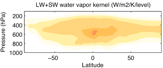
Average TOA feedback kernels, calculated with CESM version 1.1.2 using PORT (Conley et al 2012). Compare with Soden et al (2008) or Block and Mauritsen (2013). Note that the temperature and water vapor kernels here are on sigma rather than pressure levels, which affects the units. (contributed by A. Pendergrass)

Radiative feedbacks in the CESM large ensemble (Kay et al 2014) calculated with the feedback kernels shown in Figure 1. (contributed by A. Pendergrass)