Water Isotopes from Satellites
Key Strengths
Key Limitations
Expert User Guidance
#General Comments
Remote-sensing observations of the water vapor isotopic composition can be used as a complementary tool to evaluate the hydrological cycle in atmospheric models.
Collocation:
Whatever the dataset used to evaluate a model, to take into account the spatio-temporal sampling biases of the data, it is preferable to collocate the model output with each of the measurements at a scale daily or shorter. To ensure that the large-scale circulation in the model is consistent with that of the data on a day-to-day basis, it is preferable to use simulations whose winds are nudged by reanalyses.
Kernel convolution:
In addition to the collocation, to take into account the sensitivity of the instruments, the model outputs need to be convolved with averaging kernels available for some of the datasets.
Clear-sky sampling bias:
All datasets sample preferentially clear-sky scenes. Even when collocating model outputs from a nudged simulation, the model might simulate cloudy conditions when the data sees clear-sky and vice versa. Therefore, in the model the clear-sky sampling bias can be under-estimated compared to the data. This effect is difficult to take into account since the definition of a cloud varies between instruments and between models.
Specific to TES:
Quality selection:
We select only retrievals for which the degree of freedom for signal is
higher than 0.5
Bias correction:
When using the TES data, a correction must be applied which decreases the deltaD by about 4 permil. This correction depends on the averaging kernels of individual measurements, as described in Lee et al 2011 and Risi et al submitted.
Sensitivity:
The sensitivity of the TES deltaD retrievals decreases as surface temperature decreases, as humidity decreases and as cloud cover increases. The sensitivity becomes very small poleward of 45°S and 45°N. When the sensitivity is small, the retrieved deltaD tends toward a constant a-priori profile which is relatively enriched. Therefore, the TES retrievals underestimate the deltaD latitudinal gradient (Risi et al submitted).
Kernel convolution:
Model outputs need to be convolved with averaging kernels, as described in Worden et al 2006, Risi et al submitted, Yoshimura et al in press, kurita et al submitted. This is crucial for a fair model-data comparison.
Specific to SCIAMACHY:
Quality selection:
To avoid potential isotopic biases related to the presence of clouds or sampling of an incomplete atmospheric column, we discard all retrievals associated with a cloud fraction higher than 10% or with a retrieved precipitable water differing from ECMWF reanalyses by more than 10% (Risi et al 2010, Risi et al submitted).
Kernel convolution:
No averaging kernel are available. We just need to calculate the total column average deltaD from the model outputs.
Specific to ACE:
Quality selection:
We discarded measurements with errors in H2O and HDO higher than the retrieved values. However, this leads to a slight bias towards measurements when H2O. In addition, we apply a 3 median average deviation filter to remove outliers (Risi et al submitted).
Kernel convolution:
ACE does not use optimal estimation, and averaging kernels are not computed. To take into account the vertical resolution of the data, we convolved the model outputs with a triangular kernel of base 3 km (Dupuy et al 2008).
Sampling:
The sampling is very sparse. In the upper troposphere, the spatial coverage is insufficient to plot maps. Only zonal averages at best can be analyzed (Risi et al submitted).
Specific to MIPAS:
Quality selection:
We discard data with the visibility flag equal to zero and with diagonal elements of the averaging kernels lower than 0.03 (Risi et al submitted).
Kernel convolution:
Model outputs need to be convolved with averaging kernels and a-priori profiles for each measurement the model is being collocated with.
Alternatively, since averaging kernels depend mainly on the tropopause height, we can use pre-computed representative averaging kernels for different tropopause height (Risi et al submitted).
Key Figures
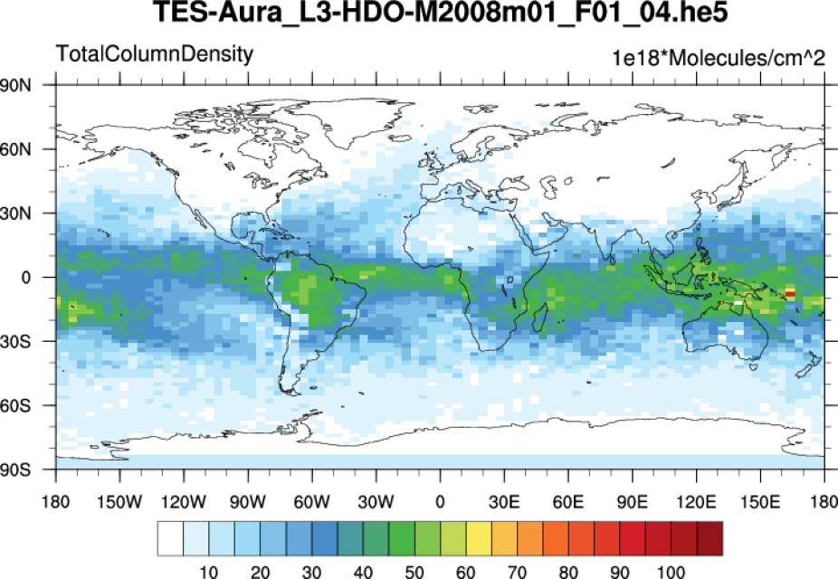
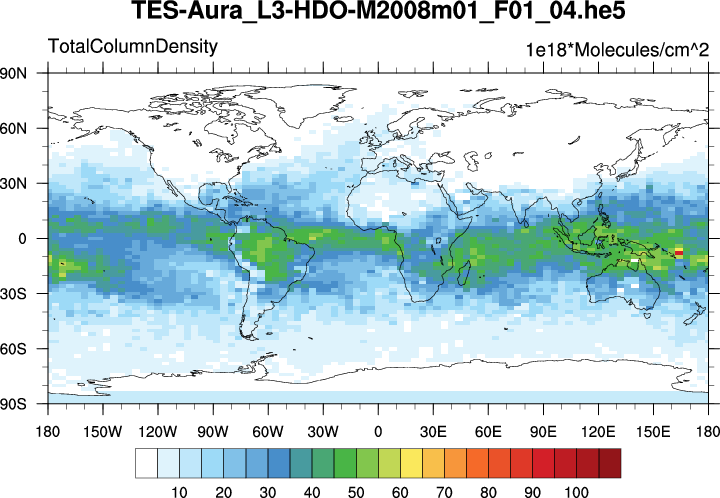
NASA TES: Total column density of HDO (January 2008).
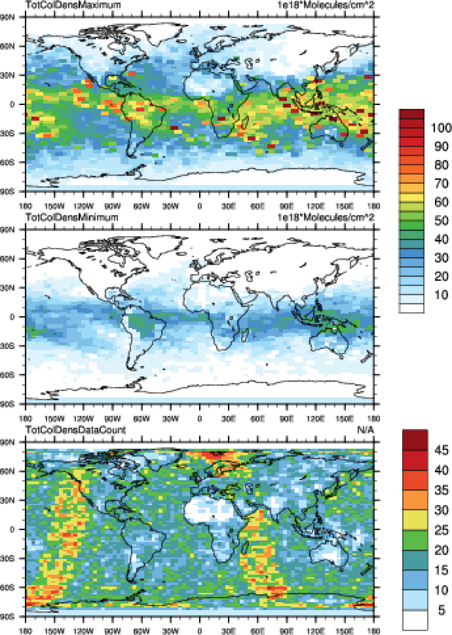
NASA TES: Minimum and Maximum total column density and the observation count (January 2008).
Other Information
satellite
Water Isotopes From Satellites
| SCIAMACHY | TES, version F04, F05 | TES profiles, TBD | ACE, v2.2_HDO_Update | MIPAS, v30_HDO5 | GOSAT | IASI | |
|---|---|---|---|---|---|---|---|
| Variable(s) | δD | δD | dD | δD | δD | δD | δD |
| Primary Input Data | shortwave infrared spectrometer on ENVISAT, total column | thermal infrared spectrometer on Aura, sensitive to mid-troposphere | thermal infrared spectrometer on Aura, sensitive to mid-troposphere | limb infrared occultation sounder, sensitive in upper troposphere | limb infrared sounder on ENVISAT, sensitive in upper troposphere | shortwave infrared spectrometer, total column | thermal infrared spectrometer, tropospheric profiles (3 independent levels) |
| Spatial Coverage | Global | Global | Global | Global, but sparse | Global | Global | Global |
| Spatial Resolution (lat x lon x vertical) |
120x20 km, total column |
5.3x8.5 km, 600hPA | 5.3x8.5 km, 3 independent tropospheric levels | limb measurement, down to 500 hPA | limb measurement, down to 400 hPA | ? | |
| missing data present? | yes | yes | yes | yes | yes | yes | yes |
| Start of record | 2003 | 2004 | 2004 | 2003 | Sept., 2002 | 2009? | ? |
| End of record | 2005 | 2011 | 211 | 2008 | March, 2004 (might be longer) | ongoing? | ? |
| Timestep (raw) | 1x per day | 2x per day, 2am & 2pm local | sunset and sunrise | 10a & 10p local time | ? | ||
| Timestep (processed) | as measured | as measured | as measured | as measured | ? | ||
| Lead Institution | European Space Agency (ESA) | NASA | NASA | Canadian Space Agency | ESA | Japan Aerospace Exploration Agency (JAXA) | ESA |
| Use restrictions | contact PI | public | contact PI | contact PI | contact PI | info forthcoming | contact PIs(note 2 main groups) |
| Data download location 1 | contact PI | NASA | available soon - contact PI | contact PI | contact PI | contact PI | contact PIs |
| Data download location 2 | |||||||
| DOI (if applicable) | |||||||
| Data format(s) available | ascii | HDF | netCDF | ascii | ascii | ? | ? |
| Are the data updated? | contact PI | yes | contact PI | contact PI | contact PI | contact PI | contact PI |
| This table last updated byInformed Guide | TES profile info is preliminary | GOSAT info is preliminary | IASI info is preliminary, and the 2 groups may produce different versions |