Tide gauge sea level data
The global sea level record from tide gauges is an important indicator of the evolution and impact of global change. Tide gauge data also capture a variety of local and regional phenomena related to decadal climate variability, tides, storm surges, tsunamis, swells, and other coastal processes. Tide gauge data are used to validate ocean models and to detect errors and drifts in satellite altimetry. Compared to satellite data, tide gauge data offer a longer record and finer temporal resolution but coarser spatial resolution. The calculation of global mean sea level from tide gauges is not straightforward due to a number of considerations, including local and regional changes in winds and ocean circulation that impact sea level, the impact of atmospheric pressure changes on sea level, the relative lack of long, continuous records, and the lack of a common datum across tide gauge sites.
Key Strengths
Used to measure climate change and climate variability at multiple temporal and spatial scales
Long record (100+ years) at many locations and high-frequency coverage
Sample water at the coastline directly, facilitating the study of tides, storm surges, and swells
Key Limitations
Many corrections to raw data are required to account for vertical land motion, regional and local variability, and atmospheric pressure
Uneven and incomplete spatial distribution that complicates calculation of the global mean
Lack a consistent global datum (benchmark) to combine tide gauge measurements from multiple locations into regional or global means
Expert User Guidance
The following was contributed by Dr. Benjamin Hamlington at Old Dominion University, and Dr. Phil Thompson at the University of Hawaii, December, 2015:
Introduction
Tide gauge sea level observations are an essential component of the global ocean observing system. Historical tide gauge data allow scientists to estimate global sea level rise since the industrial revolution, which is a powerful indicator of both the trajectory and impact of anthropogenic-driven increases to global mean temperature [e.g. Douglas, 1991; Church et al., 2011]. Tide gauges also capture a variety of oceanic and geodetic phenomena at many time and space scales. Examples include tides, decadal climate variability (e.g., the Pacific Decadal Oscillation), planetary waves, storm surge, tsunamis, and glacial isostatic adjustment. In addition to process-oriented research, tide gauge data are assimilated into and provide validation for ocean models [e.g. Carton et al., 2005; Balmaseda et al., 2013], used to detect errors and drifts in satellite altimetry [e.g. Mitchum et al., 1998; Watson et al., 2015], and are a key component of tsunami warning systems [e.g. Titov et al., 2005].
What is a tide gauge?
A tide gauge is an instrument that measures water level relative to a fixed point on land. The fixed point is referred to as a benchmark, and it is a crucial component of any tide gauge installation. The height of the tide gauge instrumentation is leveled to the benchmark with high-precision survey techniques, and the primary benchmark is generally tied to other benchmarks in the area to monitor the stability of the land and gauge.
The most common type of tide gauge is mechanical in nature and consists of a float in a stilling well attached to a data recorder. In the past, the recorder was a pen that moved with the height of the float across long scrolls of paper; modern recorders are digital. A stilling well is a vertical cylinder with a small hole in its side that acts as a mechanical filter as it fills and drains with changes in surrounding water level. The well prevents turbulent motion of the ocean surface from disturbing the float.
Other types of tide gauges include pressure sensors, acoustic gauges, and radar gauges. Pressure sensors rest on the ocean floor and measure the weight of the water above them, which can be converted to height using the water density. Acoustic and radar gauges measure the travel time or phase change of acoustic and radar pulses sent from the sensor and reflected vertically from the sea surface. At the time of writing, radar gauges are the preferred instrumentation for new installations.
Considerations when interpreting tide gauge data
3.1 Vertical land motion
Tide gauges measure relative sea level, which is the height of the water relative to the height of the land. This means that tide gauge sea level observations reflect vertical motion of both the sea surface and the coastline. For example, extraction of hydrocarbons in the ground near Galveston, TX is causing the land to subside in the region. The local tide gauge measures the land subsidence as additional long-term relative sea level rise on top of the increase due to increasing global mean temperature. Considering the effect of vertical land motion (VLM) is particularly important when calculating long-term sea level trends from tide gauges.
For some applications, it is necessary to correct for vertical land motion in tide gauge observations. One of the most important sources of VLM is glacial isostatic adjustment (GIA), which is the ongoing slow rebound of the Earth’s crust after removing the weight of ancient ice that existed during the last glacial maximum [e.g. Peltier, 1998]. This process manifests as long-term linear trends in tide gauge observations, and GIA models can be used to remove the GIA trends from the tide gauge data [e.g. Peltier, et al., 2015].
It may be possible to correct for other sources of VLM (seismic motion, subsidence, etc.) using Global Positioning System (GPS) measurements. This should be done with caution, however, because GPS captures time-dependent processes (unlike GIA, which is approximately constant for time-scales on the order of 100 years). The current rate of VLM measured by a GPS may not be the rate of land motion over the entire tide gauge record. Land motion can also vary over short distances, and using GPS data from a receiver that is not precisely co-located with a tide gauge may lead to erroneous conclusions.
3.2 Regional and local variability
Global sea level rise is just one of many ocean processes captured in tide gauge sea level records. Local and regional changes in winds and ocean circulation also affect sea level. The difference is that long-term sea level rise is mostly permanent on human time-scales, while sea level change due to wind and circulation is temporary. For example, mean sea level along the California coast did not rise during the last two decades [e.g., Thompson et al., 2014], but this does not mean sea level rise is unimportant in the region. Instead, recent strengthening of Pacific trade winds has increasingly pushed ocean water to the west and away from California. In contrast, sea level rise in California was faster than the global average during prior decades when the trades showed a weakening trend. When the recent strengthening of Pacific trades reaches a maximum and begins to decrease, scientists expect sea level rise in California to resume. It is thus imperative to consider the effect of local and regional wind and circulation when formulating conclusions based on tide gauge data.
3.3 Inverted barometer
Sea level at any particular location is affected by the weight of the atmosphere above that location. High atmospheric pressure in one area displaces ocean water toward areas of low atmospheric pressure. This isostatic process is called the inverted barometer effect, and it can account for more than 50% of the variability in monthly mean sea level in some places. The effect must be removed a priori when using tide gauge data to study dynamical processes in the ocean, such as circulation and waves. Correcting tide gauge data for inverted barometer is straightforward, as a 1mb increase in atmospheric pressure at sea level (SLP) corresponds to approximately 1mm of sea level fall [Ponte, 2006]. Of course, the quality of this correction depends on the quality of the SLP record, and gridded SLP products may not be adequate in data-poor areas prior to the advent of satellite meteorology in the 1970s.
3.3 Global mean sea level
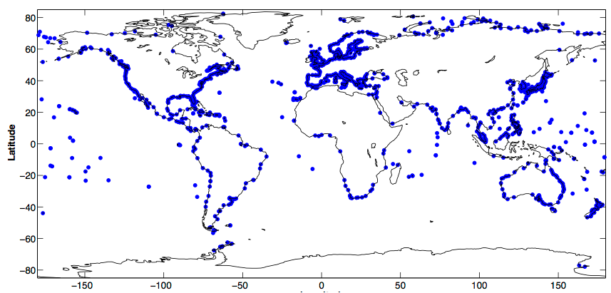
Calculating global mean sea level (GMSL) from historical tide gauge observations is a challenging problem. First, tide gauges are necessarily located along continental and island coasts, and the ocean interior is poorly sampled. Second, the configuration of the global network varies substantially in both space and time (Figure 1). There are a few long records that provide mostly continuous time series since the early 19th century, but the majority of tide gauge records are much shorter. The number of tide gauges increases considerably after World War II, reaching a maximum during the 1980s [Holgate et al., 2013]. There is also significant clustering of gauges around heavily populated areas – particularly in the Northern Hemisphere (Figure 1, bottom). These characteristics of the tide gauge network are problematic, because sea level does not change uniformly due to the regional and local response of sea level to wind and ocean circulation discussed above. If not handled properly, the non-uniform spatial and temporal sampling can lead to aliasing of the regional and local variability into estimates of GMSL [e.g. Hamlington and Thompson, 2015]. One way to address this issue is to combine the long time series of sea level from tide gauges with the shorter and more spatially complete observations from satellite altimetry (see Section 4).
Another important consideration for calculating global mean sea level from tide gauges is the lack of a consistent global datum. Tide gauges are tied to a local datum (the benchmark, see above) that requires a detailed and carefully documented history to be useful for sea level applications. While this is done on a local level, there is no consistency on larger scales. The lack of a consistent datum is important when trying to combine tide gauges at different locations. Simply averaging tide gauge records together to form a global mean is not possible, as the lack of common datum will contaminate calculations of the global average.
Tide gauges and satellite altimetry: comparative strengths and weaknesses
Tide gauges and satellite altimetry are complimentary datasets, and both are necessary to observe the complete spectrum of processes that lead to sea level variability. Since 1993, satellite altimeters have provided continuous, near-global (± 66ºN) measurements of sea surface height. These measurements provide definitive estimates of global mean sea level rise during recent decades (~3.2 mm/year from 1993 to present) with much less uncertainty than the global rate derived from tide gauges. Tide gauges, on the other hand, provide the long-term context that is necessary to interpret the short satellite record.
In general, tide gauges are superior in the temporal domain, while satellite altimetry is superior in the spatial domain. As noted above, tide gauge records are often much longer than the satellite record, but they also provide much higher temporal resolution. Tide gauge heights are often collected with a resolution on the order of minutes, and the data are publically available with hourly latency. In contrast, satellite altimeters are limited by the return period of their orbit, which for the current generation of NASA altimeters is about 10 days. Tide gauges also sample water level at the coastline directly, while altimeters perform poorly within 50-100 km of the coast due to issues with the wet troposphere correction near land. For these reasons tide gauge observations are necessary for studying high-frequency coastal processes, such as tides, storm surge, swell energy, and shelf waves. Quantifying and understanding these processes is essential for the purposes of planning, adaptation and mitigation of sea level rise impacts.
Techniques have been developed to combine tide gauge and altimetry data to obtain optimal estimates of historical sea level change [e.g. Chambers et al., 2002; Church and White et al., 2004; 2006, 2011; Ray and Douglas, 2011]. Spatial patterns of recent sea level change from altimetry are projected onto variability in the long sea level records from tide gauges to ‘reconstruct’ estimates of the global sea level field prior to the availability of satellite data. These methods attempt to overcome the shortcomings of each dataset by combining their strengths.
Data centers
The primary international authority on the collection, quality-control, and archiving of tide gauge sea level observations is the Global Sea Level Observing System (GLOSS; http://www.gloss-sealevel.org), which is an international program established by the World Meteorological Organisation (WMO) and the UNESCO Intergovernmental Oceanographic Commission (IOC). The core of the GLOSS program is an international group of data centers that provide a suite of cross-referenced sea level datasets for a variety of research and operational applications. The various centers that participate in GLOSS and the data services they provide are briefly outlined below. Extensive documentation for obtaining and using tide gauge data is available from the GLOSS and partner websites.
The Permanent Service for Mean Sea Level (PSMSL; http://www.psmsl.org/) provides a global archive of monthly and annual quality-controlled sea level records. Based on the quality of the benchmark history, PSMSL categorizes tide gauge records into one of two datasets: the Revised Local Reference (RLR) dataset, and the Metric dataset. Records in the RLR dataset have a well-defined and internally consistent benchmark history, which makes these records suitable for studies of long-term sea level change. The Metric records, on the other hand, are missing complete benchmark histories, and PSMSL advises that these gauges are not to be used for climate studies.
High-frequency tide gauge data (hourly and daily) are available from the University of Hawaii Sea Level Center (UHSLC; http://uhslc.soest.hawaii.edu). High-frequency data is not available for all records in the PSMSL database, because many agencies do not archive the high-frequency data or are not willing to provide it to the international community. Two levels of quality control are provided by the UHSLC. Research Quality data is updated annually and has been fully vetted for datum shifts, drifts, and unphysical anomalies. Fast-Delivery data is updated every 1-2 months, but has received only minimal quality-control and is best suited for operational applications and satellite calibration.
Real-time, raw tide gauge data for tsunami monitoring and other purposes are available from the IOC sea level monitoring website (http://www.ioc-sealevelmonitoring.org) maintained by the Flanders Marine Institute in Belgium (VLIZ; http://www.vliz.be). The monitoring website provides data for download, as well as interactive sea level graphs for each station that update as more data becomes available.
GLOSS considers GPS estimates of vertical land motion an essential sea level variable. The GLOSS data center for GPS time series at tide gauge locations (where existing) is Système d'Observation du Niveau des Eaux Littorales (SONEL; http://www.sonel.org). GPS time series are available for download from the SONEL website.##
Cite this page
Acknowledgement of any material taken from or knowledge gained from this page is appreciated:
Hamlington, Benjamin &, Thompson, Phil & National Center for Atmospheric Research Staff (Eds). Last modified "The Climate Data Guide: Tide gauge sea level data.” Retrieved from https://climatedataguide.ucar.edu/climate-data/tide-gauge-sea-level-data on 2026-07-21.
Citation of datasets is separate and should be done according to the data providers' instructions. If known to us, data citation instructions are given in the Data Access section, above.
Acknowledgement of the Climate Data Guide project is also appreciated:
Schneider, D. P., C. Deser, J. Fasullo, and K. E. Trenberth, 2013: Climate Data Guide Spurs Discovery and Understanding. Eos Trans. AGU, 94, 121–122, https://doi.org/10.1002/2013eo130001
Key Figures
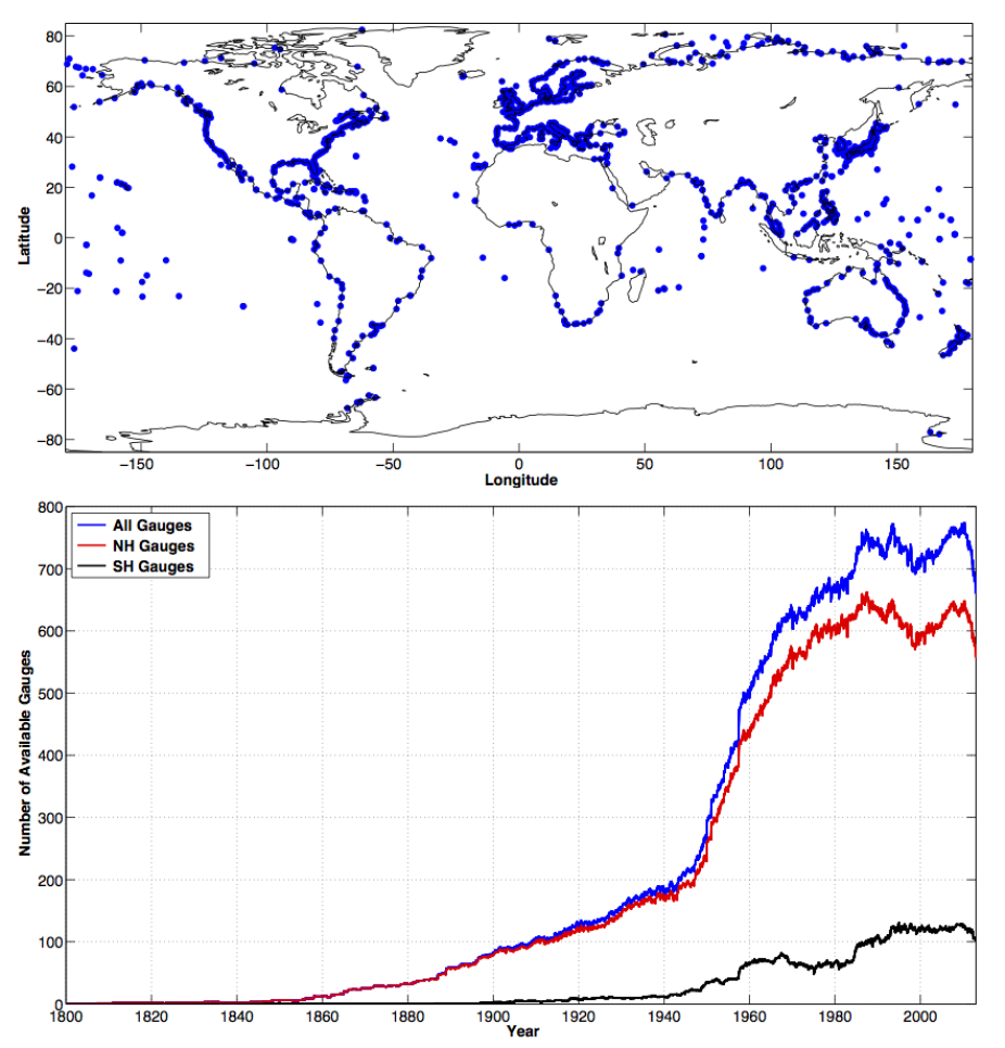
Top: Spatial distribution of the 1420 tide gauges in the PSMSL RLR dataset. Bottom: Number of available tide gauges in the PSMSL RLR dataset through time (blue). Available gauges for the Northern Hemisphere (red) and Southern Hemisphere (black) is also shown for comparison. (contributed by B. Hamlington)
Other Information
- Balmaseda, M. A., Mogensen, K. and Weaver, A. T. Evaluation of the ECMWF ocean reanalysis system ORAS4. Q.J.R. Meteorol. Soc., 139: 1132–1161, (2013).
- Carton, J. A., Giese, B.S., and Grodsky, S.A., Sea level rise and the warming of the oceans in the Simple Ocean Data Assimilation (SODA) ocean reanalysis, J. Geophys. Res., 110, C09006, (2005).
- Chambers, D.P., Melhaff, C.A., Urban, T.J., Fuji, D., Nerem, R.S. Low-frequency variations in global mean sea level: 1950-2000. J. Geophys. Res. 107, 3026, (2002).
- Church, J.A., White, N.J., Coleman, R., Layback, K., Mitrovica. J.X. Estimates of the regional distribution of sea level rise over the 1950-2000 period, J. Climate 17, 2609-2625 (2004).
- Church, J.A., White, N.J. A 20th century acceleration in global sea level rise, Geophys. Res. Lett. 36, L040608, (2006).
- Church, J.A., White, N.J. Sea-Level Rise from the Late 19th to the Early 21st Century. Surveys in Geophysics 32-4, 585-602 (2011).
- Douglas, B. C. Global sea level rise, J. Geophys. Res., 96(C4), 6981–6992, (1991).
- Hamlington, B. D., and P. R. Thompson, Considerations for estimating the 20th century trend in global mean sea level. Geophys. Res. Lett., 42, 4102–4109, (2015).
- Holgate, S.J., et al. New Data Systems and Products at the Permanent Service for Mean Sea Level. Journal of Coastal Research, 29(3), pp. 493, (2013).
- Mitchum, G.T. Monitoring the Stability of Satellite Altimeters with Tide Gauges. J. Atmos. Oceanic Technol., 15, 721–730, (1998).
- Ponte, R.M., Low-Frequency Sea Level Variability and the Inverted Barometer Effect. J. Atmos. Oceanic Technol., 23, 619–629. (2006).
- Peltier W.R., Postglacial Variations in the Level of the Sea: Implications for Climate Dynamics and Solid-Earth Geophysics. Reviews of Geophysics, 36(4),603-689, (1998).
- Peltier, W.R., Argus, D.F. and Drummond, R. Space geodesy constrains ice-age terminal deglaciation: The global ICE-6G_C (VM5a) model. J. Geophys. Res. Solid Earth, 120, 450-487, (2015).
- Ray, R., and B. Douglas, Experiments in reconstructing twentieth-century sea levels, Prog. Oceanogr., 91, 496–515, (2011).
- Thompson, P.R., Merrifield, M.A., Wells, J.R., Chang, C.M. Wind-Driven Coastal Sea Level Variability in the Northeast Pacific. J. Climate, 27, 4733–4751, (2014).
- Titov, V.V., et al. Real-Time Tsunami Forecasting: Challenges and Solutions. In Developing Tsunami-Resilient Communities, 41–58. Springer Netherlands, (2005).
- Watson, C.S., White, N.J., Church, J.A., King, M.A. Burgette, R.J., Legresy, B., Unabated Global Mean Sea-Level Rise over the Satellite Altimeter Era. Nature Climate Change, 5 (6). (2015).