Ocean temperature analysis and heat content estimate from Institute of Atmospheric Physics
The Institute of Atmospheric Physics (IAP) ocean temperature analysis features global coverage of the oceans, at 1° x1° horizontal resolution on 41 vertical levels from 1-2000m, and monthly resolution from 1940 to present. As such, it is aimed at studies of climate variability and change, from large regional to global scales, on timescales of months to decades. The primary input data are bias-corrected (for depth error, temperature error and probe type) XBT measurements from the World Ocean Database. Model simulations were used to guide the mapping from point measurements to the grid, while sampling error was estimated by sub-sampling the ARGO data at the locations of the earlier observations. The dataset has been used to estimate ocean heat content change since 1940, which compares favorably with the top-of-atmosphere radiative imbalance since 1985.
Key Strengths
Global, gridded dataset of ocean subsurface temperature
Uses a community recommended XBT bias correction approach
Error estimates provided
Key Limitations
Does not resolve small-scale ocean features such as eddies
Prior to the ARGO era, sampling uncertainty is of similar magnitude to interannual variability
Data from 1940-1955 should be used with caution (large uncertainty, and the reconstruction is shifted to CMIP5 model ensemble mean)
Cheng L., K. Trenberth, J. Fasullo, T. Boyer, J. Abraham, J. Zhu, 2017: Improved estimates of ocean heat content from 1960 to 2015, Science Advances, 3, e1601545.
Expert Developer Guidance
The following was contributed by Dr. Lijing Cheng, Institute of Atmospheric Physics at the Chinese Academy of Sciences, May, 2017:
A gridded ocean temperature dataset with complete global ocean coverage is a highly valuable resource for the understanding of climate variability and change. The Institute of Atmospheric Physics (IAP) provides a new objective analysis of historical ocean subsurface temperature since 1940 for the upper 2000m through several innovative steps. The first was to use an updated set of past observations that had been newly corrected for biases (e.g., in XBTs). The XBT bias was corrected by CH14 scheme (Cheng et al. 2014), which is recommended by the XBT community (Cheng et al. 2016). The second was to use co-variability between values at different places in the ocean and background information from a number of climate models that included a comprehensive ocean model (Cheng and Zhu, 2016; Cheng et al. 2017). The third was to extend the influence of each observation over larger areas, recognizing the relative homogeneity of the vast open expanses of the southern oceans. Then the observations were also used to provide finer scale detail. Finally, the new analysis was carefully evaluated by using the knowledge of recent well-observed ocean states, but subsampled using the sparse distribution of observations in the more distant past to show that the method produces unbiased historical reconstruction (Cheng et al. 2017). The method works well back to the late 1950s but prior to then there are too few observations to make reliable ocean state estimates.
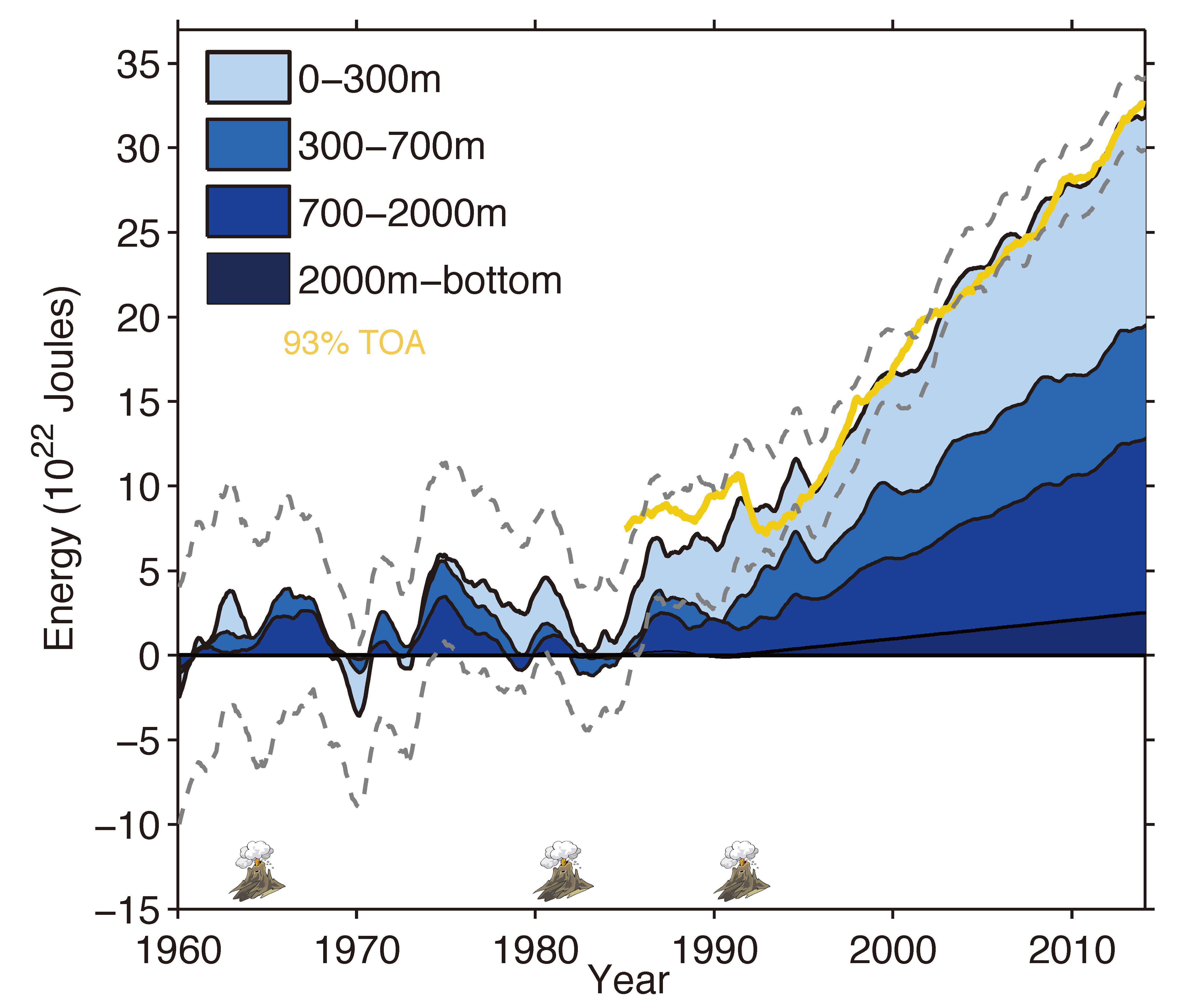
Ocean heat content (OHC) change is a fundamental indicator of global warming, since the ocean stores more than 90% of the earth’s energy increase (von Schuckmann et al. 2016). Accurate assessment of OHC change is a key task and a key challenge in the climate community (Cheng et al. 2015; Boyer et al. 2016). Based on the IAP ocean temperature analysis, we provide a new OHC estimate with an unbiased mean sampling error. The reconstructed OHC variability on decadal and multi-decadal timescales (signal) can be reliably distinguished from sampling error (noise) with signal-to-noise ratios larger than 3. The temperature variation on inter-annual scale is smaller (or comparable, S/N ratio ~ 1) than the noise before Argo era, due to insufficient sampling. The inferred integrated EEI is greater than reported in previous assessments, but consistent with a reconstruction of the radiative imbalance at the top-of-atmosphere since 1985.
What are the key differences in methods used to create IAP data and its peer datasets (for example: WOA by NCEI, EN4 by Hadley Center, Ishii data by JMA)? Here we briefly discuss two major techniques used to create these datasets including XBT bias correction and mapping method. There are major error sources in OHC calculation as discussed in Boyer et al. 2016. We will also highlight the “subsample test” to quantify the accuracy of the reconstruction, which was not done by other peer datasets except IAP data.
(1). Correction to XBT bias. XBT bias can significantly impact the OHC estimates, especially for decadal and long-term changes. IAP data corrects XBT bias by using the Cheng et al. 2014 method (CH14), which is a recommended method by XBT community. CH14 corrects both depth error and pure temperature error, and also takes accounts of the influence of ocean temperature, manufacturer and probe type. WOA uses the Levitus et al. 2009 (L09) scheme, which corrects only XBT temperatures; EN4 provides several different versions of products by using L09 and Gouretski & Reseghetti 2010 (GR10) respectively. GR10 provides correction to both depth error and temperature error for the main XBT probe types. Ishii data used the Ishii and Kimoto (2009) method, which attributes XBT bias only to depth error.
(2). Mapping method. The mapping method defines how data gaps are filled and the reconstructed field is smoothed. The covariance defines the correlations of temperature changes among different grid boxes, which is vital in an objective analysis. Previous products (WOA, EN4 and Ishii) have parameterized the background error correlation between two points as a function which decays in an exponential-like manner with the distance separating the points. This parameterized correlation is always isotropic, however, the covariance should be flow-dependent in the real ocean. The over-simplified covariance is one major error source in ocean temperature reconstructions. The IAP product uses an Ensemble Optimum Interpolation method combined with covariance from CMIP5 multi-model simulations. The models have the capability to simulate the general ocean circulation and could provide a better representation of the covariance. Using the ensemble strategy effectively reduces the impact of model bias in each single model, therefore, the IAP mapping technique provides a best guess on the covariance based on a combination of climate model simulations.
In addition to mapping, a localization strategy is always applied due to the inaccuracy of the remote covariance, which assumes that only data within a spatial area can be used during the analysis of a grid cell. The size of the area is defined by the influencing radius. WOA/Ishii/EN4 method uses a radius less than 900km. Instead IAP uses 20 degrees for an influencing radius within 0-700m (25 degrees for 700-2000m). The large fractional coverage helps ensure that a near-complete global reconstruction can be reached, so the technique will not bias the reconstructed field toward the first-guess field in data sparse regions.
(3). Subsample test to evaluate the analysis. Quantification of the reliability of the reconstruction is an important step for a product. A subsample test, in which subsets of data in the data-rich Argo era are co-located with locations of earlier ocean observations, is performed to quantify the sampling error. The subsample test is defined as the difference between the reconstructed and “truth fields”. The truth field is taken to be a set of the gridded averaged temperature anomalies during the Argo era. Each truth field is subsampled according to the locations of historical observations and mapped to get the reconstructed fields. The IAP product is evaluated by this subsample test, showing an unbiased mean sampling error and with ocean temperature (or OHC) variability on decadal and multi-decadal timescales that can be reliably distinguished from sampling error. In addition, temperature (or OHC) changes in six major ocean basins are reliably reconstructed on decadal timescales. However, the inter-annual variations in the pre-Argo era are of comparable magnitude to sampling errors, but the current Argo system begins to allow for a resolution of inter-annual temperature (or OHC) variability. A similar subsample test is highly recommended in the future in the evaluation of an ocean analysis.##
Cite this page
Acknowledgement of any material taken from or knowledge gained from this page is appreciated:
Cheng, Lijing & National Center for Atmospheric Research Staff (Eds). Last modified "The Climate Data Guide: Ocean temperature analysis and heat content estimate from Institute of Atmospheric Physics.” Retrieved from https://climatedataguide.ucar.edu/climate-data/ocean-temperature-analysis-and-heat-content-estimate-institute-atmospheric-physics on 2026-02-26.
Citation of datasets is separate and should be done according to the data providers' instructions. If known to us, data citation instructions are given in the Data Access section, above.
Acknowledgement of the Climate Data Guide project is also appreciated:
Schneider, D. P., C. Deser, J. Fasullo, and K. E. Trenberth, 2013: Climate Data Guide Spurs Discovery and Understanding. Eos Trans. AGU, 94, 121–122, https://doi.org/10.1002/2013eo130001
Key Figures
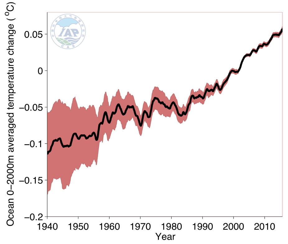
Figure 1. 0-2000m averaged temperature change since 1940 along with uncertainty estimates (95% confidence interval). (contributed by L Cheng)

Figure 2. Ocean energy budget based on IAP ocean temperature analysis. The 93% of the energy imbalance observed from the top of atmosphere is shown in yellow. OHC change below 2000m is from Purkey and Johnson 2010. (contributed by L Cheng)
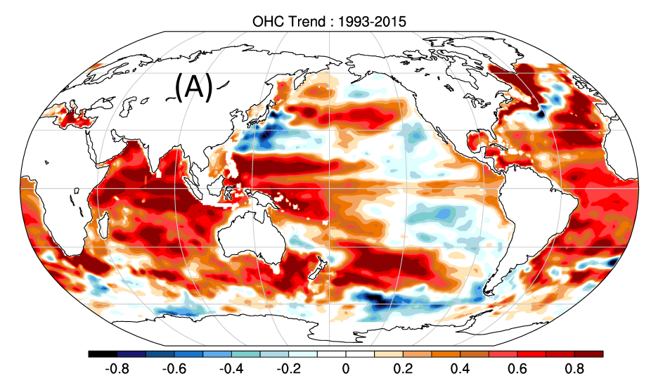
Figure 3. Trend of ocean heat content change from 1993 to 2015 (unit: 108 J/m2). (contributed by L Cheng)
Other Information
- Cheng L., K. Trenberth, J. Fasullo, T. Boyer, J. Abraham, J. Zhu, 2017: Improved estimates of ocean heat content from 1960 to 2015, Science Advances, 3, e1601545.
- Cheng L. and coauthors, 1. 2016: XBT Science: assessment of instrumental biases and errors, Bulletin of the American Meteorological Society, 97, 924-933, doi: http://dx.doi.org/10.1175/BAMS-D-15-00031.1.
- Cheng L. and J. Zhu, 2016, Benefits of CMIP5 multimodel ensemble in reconstructing historical ocean subsurface temperature variation, Journal of Climate, 29(15), 5393–5416, doi: 10.1175/JCLI-D-15-0730.1.
- Cheng L., J. Zhu, R. Cowley, T. P. Boyer and S. Wijffels, 2014: Time, probe type and temperature variable bias corrections on historical expendable bathythermograph observations. Journal of Atmospheric and Oceanic Technology, 31(8), 1793-1825.
- Cheng L. and J. Zhu, 2015: Influences of the choice of climatology on ocean heat content estimation, Journal of Atmospheric and Oceanic Technology. 32(2), 388-394.
- Cheng, L., J. Zhu, and J. Abraham, 2015: Global upper ocean heat content estimation: recent progress and the remaining challenges. Atmos. Oceanic Sci. Lett., 8, 333-338.
- Purkey, S., and G. Johnson, 2010: Warming of Global Abyssal and Deep Southern Ocean Waters between the 1990s and 2000s: Contributions to global heat and sea level rise budgets. J. Climate, 23, 6336-6351.
- von Schuckmann, K. and Coauthors, 2016: An imperative to monitor Earth’s energy imbalance. Nat. Climate Change, 6, 138–144.
- Boyer, T., C. Domingues, S. Good, G. Johnson, J. Lyman, M. Ishii, V. Gourestki, N. Bindoff, J. Church, R. Cowley, J. Willis, S. Wijffels, 2016: Sensitivity of global ocean heat content estimates to mapping methods, XBT bias corrections, and baseline cl
- Gouretski, V., F. Reseghetti, On depth and temperature biases in bathythermograph data: Development of a new correction scheme based on analysis of a global ocean database. Deep-Sea Research I 57, 812-833 (2010)
- Levitus, S., J. I. Antonov, T. P. Boyer, R. A. Locarnini, H. E. Garcia, A. V. Mishonov, Global ocean heat content 1955-2008 in light of recently revealed instrumentation problems. Geophys. Res. Lett. 36, L07608 (2009).
- Ishii, M., M. Kimoto, Reevaluation of historical ocean heat content variations with time-varying XBT and MBT depth bias corrections. J. Oceanogr. 65, 287-299 (2009)