Cloud Dataset Overview
Clouds cover about 70% of the earth's surface. They are important components of the cliimate's water and energy budgets. Historically, cloud reports have come from station or ship observations. The satellite observation era, beginning in the 1980’s and spanning now more than 30 years, allows to capture clouds and their properties over the entire globe and across a wide range of temporal and spatial scales.
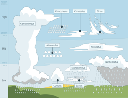
Figure 1 illustrates cloud types distinguished by cloud base height and morphology, as initially classified by surface observers. Cloud morphology, stratiform or cumuliform, indicates formation in stable or turbulent air. The International Satellite Cloud Climatology Project (ISCCP; Rossow and Schiffer 1991, 1999) adapted this cloud type classification by using cloud top pressure (CP) and optical depth (COD).
ISCCP cloud products were designed to characterize essential cloud properties and their variations on all key time scales to elucidate cloud dynamical processes and cloud radiative effects. Their success has been shown in many published analyses, also in combination with other observations. While ISCCP, the cloud data record of the GEWEX project, emphases diurnal sampling by using multi-spectral imager data from a combination of geostationary and Sun-synchroneous orbiting (SSO) weather satellites, more recent global cloud data records have been developed from various instruments onboard SSO satellites.
The GEWEX cloud assessment (2005-2012, Stubenrauch et al. 2012, 2013) completed the first coordinated intercomparison of publicly available, global cloud products. Cloud properties retrieved from measurements of multi-spectral imagers (ISCCP, PATMOS-x, MODIS-ST, MODIS-CE), IR sounders (HIRS-NOAA, TOVS Path-B, AIRS-LMD), multi-angle multi-spectral imagers (ATSR-GRAPE, MISR, POLDER) and active lidar (CALIPSO-ST, CALIPSO-GOCCP) have been included in the GEWEX Cloud Assessment Database, which provides monthly statistics on 1° latitude x 1° longitude grid in netCDF files arranged by cloud property, year, and observation time of day.
Key Strengths
Cloud properties derived from space observations provide long-term global data of cloud properties including cloud amount, height, temperature, and radiative and bulk microphysical properties
Synergy of different variables and data sets provide invaluable potential for improving our understanding of cloud processes
Long, gridded data enable characterizations of geographical patterns, seasonal and interannual variability
Key Limitations
Monitoring long-term climate variability is difficult with these data sets. Since there are systematic variations of cloud properties with location on the globe, time of day and season, variations in sampling can introduce changes that are not driven by climate.
Observed cloud data cannot necessarily be compared "apples to apples" with cloud properties estimated by climate models; use of cloud simulator packages like COSP is encouraged.
The conversion among cloud pressure, temperature and height requires atmospheric temperature profiles from ancillary data, leading to additional uncertainties.
Stubenrauch C. J., W. B. Rossow, S. Kinne, S. Ackerman, G. Cesana, H. Chepfer, L. Di Girolamo, B. Getzewich, A. Guignard, A. Heidinger, B. C. Maddux, W. P. Menzel, P. Minnis, C. Pearl, S. Platnick, C. Poulsen, J. Riedi, S. Sun-Mack, A. Walther, D. Winker, S. Zeng, and G. Zhao, Assessment of Global Cloud Datasets from Satellites: Project and Database initiated by the GEWEX Radiation Panel. Bull. Amer. Meteor. Soc., 94, 1034-1049, doi: https://doi.org/10.1175/BAMS-D-12-00117.1 (2013)
In addition, the individual data sets should be referenced and the Climserv Data Center of IPSL/CNRS should be acknowledged.
http://climserv.ipsl.polytechnique.fr/gewexca/index-2.html
- The GEWEX Cloud Assessment Database, created by the participating teams (see Technical Notes), contains monthly means, variability and distributions of many cloud properties, also stratified by height and thermodynamic phase
- Link to description and download of individual datasets that were used in the database (see also Technical Notes)
Expert User Guidance
The following was submitted by Dr. Claudia Stebenrauch, CNRS, LMB, France, in June 2018:
General Strengths and Weaknesses
KEY STRENGTHS
Cloud properties derived from space observations are extremely valuable for climate studies and model evaluation:
- long-term global data of cloud properties (amount, height, temperature, radiative and bulk microphysical properties, across a wide range of spatial and temporal scales
- geographical patterns, seasonal and interannual variability
- Active lidar, IR sounding and IR spectral differences are powerful for thin cirrus identification (with decreasing sensitivity from the former to the latter).
- Visible information (during daytime) is more important for the detection of low-level clouds.
- synergy of different variables and data sets provide invaluable potential for improving our understanding of cloud processes
- reduction of uncertainties and further advances by analyzing statistics of mesoscale cloud regimes or weather states, organized according to similar distributions in cloud pressure and optical depth, or of cloud systems constructed from individual cloud measurements according to similar height
KEY LIMITATIONS
- Biases are scene related (e.g. nighttime, thin cirrus overlaying low-level clouds, highly reflective or cold surfaces) and depend on instrument spectral domain and retrieval methodology
- The ‘radiometric cloud height’ may lie several hundred m’s to a couple of km’s below the physical top, when the cloud top is diffuse (optical depth increases slowly toward cloud base).
- The conversion among cloud pressure, temperature and height requires atmospheric temperature profiles from ancillary data, leading to additional uncertainties.
Satellite sensors
Multi-spectral imagers are radiometers that measure reflected, emitted and scattered radiation at a few discrete wavelengths, usually from the solar to thermal infrared spectrum. Nadir viewing with cross-track scanning capabilities, they have a spatial resolution from about 0.5 to 7 km (at nadir) and are the only sensors aboard geostationary weather satellites.Multi-spectral imagers aboard SSO satellites are the Advanced Very High Resolution Radiometer (AVHRR, with 5 spectral channels) and the MODerate resolution Imaging Spectroradiometer (MODIS with 36 spectral channels).
IR sounders use IR channels along the CO2 absorption band to determine cloud height and emissivity. The variable atmospheric opacity of the many channels of these IR sounding instruments allows a reliable identification of cirrus (semi-transparent ice clouds), day and night. The operational High resolution Infrared Radiation Sounder (HIRS, with 19 channels in the IR) is a multi-channel radiometer, whereas the Atmospheric Infrared Sounder (AIRS) and Infrared Atmospheric Sounding Interferometer (IASI) are infrared spectrometers. Their spatial resolution is about 15 km (at nadir). MODIS also has a few channels similar to those of HIRS.
Multi-angle, multi-spectral imagers make measurements of the same scene with different viewing angles, allowing a stereoscopic retrieval of cloud top height. Together with the use of polarization the cloud thermodynamic phase can be determined(since non-spherical ice particles depolarize the reflected light less than liquid droplets). The Multi-angle Imaging SpectroRadiometer (MISR, with 4 solar spectral channels and 9 views) and a sensor using POLarization and Directionality of the Earth’s Reflectances (POLDER, with 8 solar sub-spectral channels (3 polarized) and up to 16 views) operate during daylight conditions, while the Along Track Scanning Radiometer (ATSR, with 7 channels exploring solar to thermal infrared spectrum and 2 views) still provides infrared information during nighttime.
Active sensors extend the measurements of passive radiometers to cloud vertical profiles. Since 2006 the CALIPSO lidar and CloudSat radar, together, determine cloud top and base heights of all cloud layers. Whereas the lidar is highly sensitive and can even detect sub-visible cirrus, its beam reaches cloud base only for clouds with an optical depth less than 3. When the optical depth is larger, the radar is still capable to provide a cloud base location.
Limb sounders, such as the spectrometer of theStratospheric Aerosol Gas Experiment (SAGE) that measures the solar occultation along the earth’s limb at 4 solar wavelengths,providegood vertical resolution (1 km) at the expense of a low horizontal resolution along the viewing path (about 200 km). On the other hand, the long path leads to detection of subvisible (very thin) cirrus.
Passive microwave imagers, like the Special Sensor Microwave Imager (SSM/I) and the Advanced Microwave Sounding Radiometer-EOS (AMSR-E), make use of spectral features sensitive to water vapor and liquid water to estimate cloud liquid water path over ocean (especially if precipitation and drizzle contamination are removed).
Cloud amount and height-stratified cloud amount
Differences in average cloud properties, especially in high-level cloud amount, are mostly explained by instrument performance to detect and/or identify thin cirrus. Active lidar measurements, IR sounding along the CO2 absorption band and methods using IR spectral differences are powerful for thin cirrus identification (with decreasing sensitivity from the former to the latter). Visible information (during daytime) is more important for the detection of low-level clouds. The largest differences in retrieved cloud properties appear in the case of thin cirrus overlying low-level clouds (sketch in Fig. 2): Whereas active lidar and IR spectral information determine the cloud properties of the cirrus (CALIPSO-ST, CALIPSO-GOCCP, HIRS-NOAA, TOVS Path-B, AIRS-LMD, MODIS-ST, MODIS-CE, PATMOS-x), IR – VIS methods (ISCCP, ATSR-GRAPE) provide the properties corresponding to a radiative mean from both clouds and VIS-only methods emphasize the clouds underneath (MISR, POLDER).
Global cloud amount (CA) is about 0.68 ± 0.03, considering clouds with COD > 0.1. CA increases to 0.74, when COD > 0.01 (CALIPSO), and decreases to 0.56 for COD > 2 (POLDER).
Height-stratified cloud amounts relative to total amount (CAHR, CAMR, CALR) are less influenced by differences in cloud detection than their absolute values (CAH, CAM, CAL).
About 40% (COD > 0.1) – 50% (COD > 0.01) of all clouds seen from above are high-level clouds. However, CAHR shows a spread from 12% to 55%. This large spread in CAHR is essentially explained by instrument performance for identifying thin cirrus, especially in cases of multi-layer cloud systems (sketch on the left in Fig. 2).
Only about 15% (±5%) of all clouds are uppermost mid-level clouds. Larger ISCCP values (27% day and 40% night) include biases due to semi-transparent cirrus overlying low-level clouds during day and in addition due to semi-transparent cirrus during night. From CALIPSO we deduced that these cases constitute about 20% of all clouds, each contributing to an overestimation of about 10% in global CAMR and an underestimation in CAHR by ISCCP.
About 40% (±3%) of all clouds are single-layered low-level clouds. Outliers are HIRS-NOAA with 26% (only one IR channel for low-level clouds), MODIS-ST with 53% (misidentification of very thin cirrus in collection 5) and MISR with 62% (good spatial resolution but only visible information). The latter can be interpreted as the amount of all low-level clouds relative to all clouds.
Reliable thin cirrus identification, also in cases of multi-layer clouds, is provided by the IR spectral information, while solar information (day) is more important for a reliable low-level cloud identification.
To illustrate the range due to differing sensor sensitivities and retrieval methodologies, Fig. 3 presents local differences between maximum and minimum CA, CAHR and CALR within six datasets (ISCCP, PATMOS-x, MODIS-ST, MODIS-CE, AIRS-LMD and TOVS Path-B). While the global range between these six datasets corresponds to only 0.08 in CA and 20% in CAHR and CALR (Fig. 1), respectively, local differences may reach 0.4 in CA (deserts and mountains) and 40-70% in CAHR and CALR (ITCZ and deserts).
Cloud height
Cloud top can be accurately determined with lidar (CALIPSO), and for optically thick clouds by the MISR stereoscopic height retrieval. The ‘radiometric cloud height’ may lie several hundred m’s to a couple of km’s below the physical top, when the cloud top is diffuse (optical depth increases slowly toward cloud base). Especially high-level clouds in the tropics have such diffusive cloud tops, leading to biases in retrieved cloud top temperature of up to 10 K. According to an analysis of ISCCP and limb-viewing observations of the Stratospheric Aerosol Gas Experiment (SAGE) (Liao et al. 1995), almost 70% of the high-level clouds in the tropics have a diffuse cloud top, leading to an average positive bias of ISCCP in cloud top pressure of about 150 hPa. At higher latitudes, only 30 - 40% of the high-level clouds are in this category, leading to an average positive bias of about 50 hPa. A comparison between AIRS and CALIPSO (Stubenrauch et al. 2010, 2017) has shown that the ‘radiometric cloud height’ corresponds approximately to the middle between cloud top and cloud base (for CEM < 0.5) or ‘apparent’ cloud base (height at which COD reaches 3). When cloud height is determined via O2 absorption (e.g. POLDER), it corresponds to a location even deeper inside the cloud.
The normalized frequency distributions in Fig. 4 show a bimodal structure, especially in the tropics. This is the reason why average values of CP (CT / CZ) may be ambiguous and why it is better to use, in addition to averages over all clouds, the height-stratified averages of the different cloud properties. The agreement in the shape of the distributions is generally better over ocean than over land. The peak position for high-level clouds in the tropics varies from 150 hPa (close to tropopause, PATMOS-X, MODIS-ST, HIRS-NOAA) to 350 hPa (POLDER). The very sharp peak of PATMOS-x seems to be suspect, though the PATMOS-x retrieval had been trained by CALIPSO data. In addition, the conversion among CP, CT and CZ requires atmospheric temperature profiles from ancillary data, leading to additional uncertainties.
Cloud optical and bulk microphysical properties
Optical properties (COD, CEM) are functions of the bulk microphysical properties, in particular of cloud water path (CWP). Effective particle sizes (CRE) influences more the spectral behaviour of emitted to reflected radiation, especially for small particles. CEM and COD are quite complementary, as CEM better resolves differences in thinner cirrus clouds, while it saturates at 1 when COD still can distinguish the optically thickest clouds. Since distributions are not Gaussian and averages depend on sub-sampling prior to retrieval, it is strongly recommended to consider normalized frequency distributions of these variables. These agree quite well, when one considers retrieval filtering or possible biases due to partly cloudy pixels and due to ice-water misidentification.
Recommendations
ISCCP is the only data set to resolve the diurnal cycle. However, high-level clouds may be misidentified as mid-level clouds in the case of thin cirrus during night and thin cirrus overlying low-level clouds during day. So far only ISCCP cloud properties have been tested by comparing resulting radiative fluxes to those determined from Earth Radiation Budget instruments, revealing excellent quantitative agreement (GEWEX Radiative Flux Assessment). The PATMOS-x data show improvement in the identification of cirrus. However, diurnal variation in cloud physical properties and seasonal variation of optical and microphysical properties show still some inconsistencies. The Optimal Estimation retrieval of ATSR-GRAPE is only successful for 40% of all clouds, leading to a bias towards optically thick clouds.
The CALIPSO lidar is the most sensitive to thin cirrus (including subvisible cirrus) and also gives information on all cloud layers within the atmosphere up to an optical depth of 3. To complement this information a coupling with the radar of the CloudSat mission is necessary, but still their instantaneous Earth coverage is very small (5%).
IR sounding methods are sensitive to thin cirrus with CEM larger than about 0.1, providing reliable cirrus properties day and night. The CO2 slicing retrieval employed by HIRS-NOAA is not applicable to low-level clouds, while a weighted c2 retrieval of TOVS Path-B and AIRS-LMD may be applied to all clouds. However, the noise for low-level clouds is larger than for the other clouds because of low radiative contrast and of coarse spatial resolution of these instruments. Bulk microphysical properties can be only determined for semi-transparent cirrus.
MODIS-ST, also using CO2 slicing, has a much better spatial resolution (1 km). However the retrieval method employed in Collection 5 led to some misidentification of very thin cirrus as low-level clouds. The retrieval has been improved for Collection 6. Optical and bulk microphysical properties are only determined for a sub-sample corresponding to clouds with optical depth > 1, and therefore their ice water path is biased high.
Monitoring long-term variations is very difficult with these data sets. Since there are systematic variations of cloud properties with location on the globe, time of day and season, variations in sampling can introduce changes. Before attributing cloud amount and cloud property changes to long-term trends in other variables, one has to investigate sampling changes and the consistency of the applied ancillary data of the particular data set used.
When comparing to climate models, observation time and view from above as well as retrieval filtering have to be taken into account. This can be achieved either by simple methods (e. g. Hendricks et al. 2010) or by more sophisticated ones, like the CFMIP (Cloud Feedback Model Intercomparison Project) Observation Simulator Package (Bodas-Salcedo et al. 2011), which consists of individual simulators, each corresponding to a specific cloud dataset (like for example ISCCP, CALIPSO, MODIS, MISR or CloudSat). However, one has to keep in mind that these simulators contain the observation biases identified by the GEWEX cloud assessment and may still include other biases.
Even though instantaneous cloud properties may not be very accurate and might include scene dependent biases, the synergy of different variables and data sets provide invaluable potential for improving our understanding of cloud processes. Another way to reduce uncertainties is by organizing statistics by mesoscale cloud regimes or weather states (e. g. Jakob and Tselioudis 2003, Tselioudis et al. 2013), according to similar distributions in cloud pressure and optical depth, or analyzing cloud systems (e. g. Machado and Rossow 1993, Protopapadaki et al. 2017). ##
Cite this page
Acknowledgement of any material taken from or knowledge gained from this page is appreciated:
Stubenrauch, Claudia & National Center for Atmospheric Research Staff (Eds). Last modified "The Climate Data Guide: Cloud Dataset Overview.” Retrieved from https://climatedataguide.ucar.edu/climate-data/cloud-dataset-overview on 2026-05-24.
Citation of datasets is separate and should be done according to the data providers' instructions. If known to us, data citation instructions are given in the Data Access section, above.
Acknowledgement of the Climate Data Guide project is also appreciated:
Schneider, D. P., C. Deser, J. Fasullo, and K. E. Trenberth, 2013: Climate Data Guide Spurs Discovery and Understanding. Eos Trans. AGU, 94, 121–122, https://doi.org/10.1002/2013eo130001
Key Figures

Figure 1: Illustration of cloud types distinguished by height and morphology, as initially classified by surface observers (Image credit: Valentin de Bruyn)
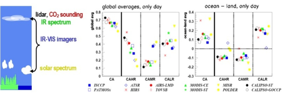
Figure 2: left: The sketch illustrates the cloud height interpretation in the case of optically thin cirrus overlying low-level clouds (less than 20% of all cloudy scenes according to CALIPSO) when using different instruments. Right: Global averages of total CA, as well as fraction of high-level, midlevel, and low-level cloud amount relative to total cloud amount (CAHR + CAMR + CALR = 1). (from Stubenrauch et al. 2012)
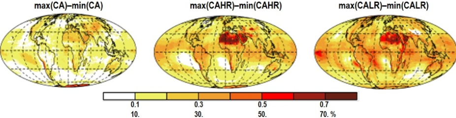
Figure 3: Regional maximum differences of CA, CAHR, and CALR within six cloud data sets (ISCCP, PATMOS-x, MODIS-ST, MODIS-CE, AIRS-LMD and TOVS Path-B). Statistics over measurements at 1:30 PM LT (3:00 PM for ISCCP). (from Stubenrauch et al. 2012)
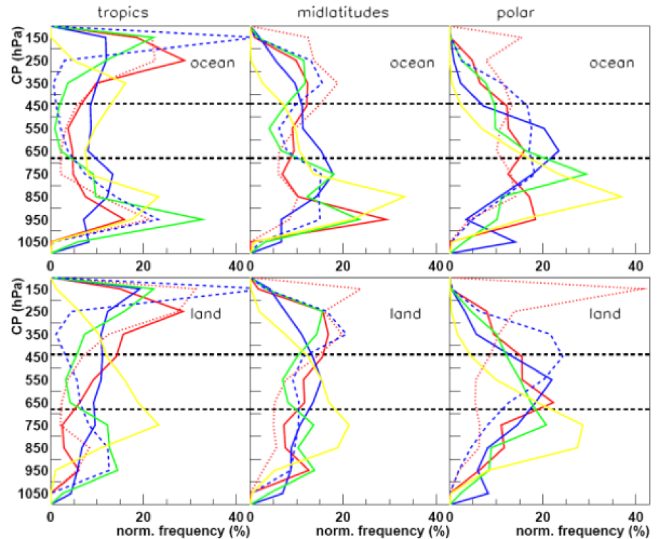
Figure 4: Normalized frequency distributions of CP in tropics (15N-15S), midlatitudes (30°-60°) and polar latitudes (60°-90°), separately over ocean and over land, during daytime. (from Stubenrauch et al. 2012)
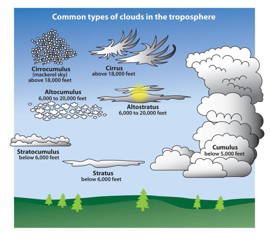
Schematic of common clouds (copyright: University Corporation for Atmospheric Research)