SST data: NOAA Optimal Interpolation (OI) SST Analysis, version 2 (OISSTv2) 1x1
Key Strengths
Expert Developer Guidance
The following was contributed by Viva F. Banzon and Richard W. Reynolds (both at NOAA/NCDC), September, 2013:
GENERAL DESCRIPTION: NOAA’s Optimum Interpolation Sea Surface temperature (OISST, also known as Reynolds’ SST) is a series of global analysis products, including the weekly OISST on a 1° grid to the more recent daily on a ¼° grid. An SST analysis is a spatially gridded product created by interpolating and extrapolating data, resulting in a smoothed complete field. OISST provides global fields that are based on a combination of ocean temperature observations from satellite and in situ platforms (i.e., ships and buoys). The input data are irregularly distributed in space and must be first placed on a regular grid. Then, statistical methods (optimum interpolation, OI) are applied to fill in where there are missing values. The methodology includes a bias adjustment step of the satellite data to in situ data prior to interpolation. SST analyses are used in a range of applications including weather forecasting, climate studies, modeling, fisheries ecology, oceanography, and as a reference field for other satellite algorithms.
VERSIONS OF OISST PRODUCED AT DIFFERENT NOAA CENTERS: The NOAA 1/4° daily OISST (version 2) is routinely produced at the National Climatic Data Center (NCDC). Version 1 is described in Reynolds et al. (2007). Version 2, released in 2008, is a minor update and is described in a web document (Reynolds, 2008). The precursor product is the 1° weekly (and daily) OISST, originally described in Reynolds and Smith (1994), and upgraded to version 2 (Reynolds et al., 2002). The National Centers for Environmental Prediction (NCEP) still produces the weekly 1° OISST, as well as a derived monthly product computed from a weighted average of the weekly OISST. It is important to understand that the OISST inputs are averaged spatially and temporally before the interpolation. Therefore, the weekly or monthly OISST cannot be produced by averaging the daily OISST. Also, methodology details have evolved over time, depending on the temporal and spatial resolution of each analysis.
DAILY 1/4° OISST VERSIONS: To serve different needs, there are two versions of the 1/4° daily OISST: “AVHRR-only” and “AVHRR+AMSR”. The AVHRR-only version uses satellite data from the infrared instrument, the Advanced Very High Resolution Radiometer (AVHRR), and is available from 1981 onward. The temporal extent of AVHRR-only (>30 years) makes it desirable for climate studies. The AVHRR+AMSR version is available from July 2002 to October 2011, and was developed to incorporate additional data from the Advanced Microwave Scanning Radiometer on the EOS platform (AMSR-E). AMSR has a lower spatial resolution (~25 km) than AVHRR but can see through clouds, resulting in significantly better spatial coverage. AVHRR is still needed because AMSR-E cannot provide reliable SSTs along the coast and in areas of precipitation. Because of AMSR-E’s almost all-weather capability, the AVHRR+AMSR version provides more accurate information in persistently cloudy areas and during hurricanes and storms. But even in cloud-free regions, the use of both infrared and microwave data can reduce systematic errors because the error characteristics of the two instruments are independent. The AVHRR+ AMSR production was discontinued when the AMSR-E antenna failed. Work is underway to reprocess with a newer version of AMSR-E data and continue the time series using newer microwave sensors: AMSR2 and WindSat (Banzon and Reynolds, 2013).
-----------------------------------------------------------------------------------------------------------------
The inputs to the daily OI version2 are:
1) For AVHRR SSTS: Pathfinder version 5.0/5.1 from 1981 to 2006, available at the National Oceanographic Data Center. Operational Navy SSTs from NESDIS from 2007 onwards. Note that a new Pathfinder version 5.2 (1981-2011)has been released and will be used in the next OISST reprocessing.
2) For AMSR SSTs: version 5 from Remote Sensing Systems. This is now superseded by version 7, which will be used in the next reprocessing. AMSR2 and WindSat data will extend the time series.
3) Sea ice concentrations (used to compute proxy SSTs at high latitudes) produced by NASA’s Goddard Space Flight Center is used up to 2004. NCEP sea ice concentrations are used from 2005 onwards. Note that the NASA team ice concentrations are now distributed by the Snow and Ice Data center and are available up to 2012.
4) Ship and buoy SSTs from the International Comprehensive Ocean and Atmosphere Dataset (ICOADS) release 2.4 (up to 2006) were used. From 2007 onwards, near real time data relayed through the Global Telecommunications System are provided by NCEP though a special arrangement. Future plans are to reprocess using more recent ICOADS release 2.5.
-------------------------------------------------------------------------------------------------------
Key strengths.
What are the key strengths of this data set?
The daily OISST product uses the same sensor type over the entire time series to keep the product more consistent over time. Thus, the AVHRR-only time series is based only on the AVHRR instrument, flown on NOAA7, 9, 11, 14, 16, 17, 18, 19, and MetopA. When available, reprocessed satellite inputs that have been better across-generation consistency are used. To be more robust, the observations are first combined to form super-observations (i.e., for each observation type, a weighted average of values within a grid box is computed).
The bias correction of satellite SSTs using in situ data is applied to compensate for any biases in the satellite data. For AVHRR, these biases occur primarily due to cloud and aerosol contamination. The worst biases occurred during the Mt Pinatubo eruption in 1992. For AMSR, biases occur primarily due to precipitation contamination. Global microwave instruments capable of measuring SST were not present before 2002. The AVHRR+AMSR version is more accurate than AVHRR-only in cloudy conditions. Both versions include error estimates to help users determine the analysis accuracy.
What are the key limitations of this data set?
The satellite bias correction relies on having adequate in situ data. In areas with sparse in situ observations, the bias correction cannot be applied. This may occur in high latitude regions, especially the Arctic.
When there are consecutive days with no observations (persistent cloudiness over a specific region), the AVHRR-only version may be unable to represent actual conditions. Areas affected by persistent cloudiness include the upwelling area off Peru, and the Gulf Stream region during the Northern Hemisphere winter.
The daily OISST does not represent a particular time of day and does not capture the diurnal variability. It is an aggregate of data for collected over the entire day.
At the marginal ice zone where satellite SST retrievals are challenging and in situ observations are rare, proxy SSTs are computed from climatological sea ice concentrations (from satellite) using an empirically derived linear regression equation with respect to SST observations. In essence, the proxy SST provides the boundary value for the analysis. The linear relation is not valid in freshwater conditions, such as in lakes or interior waters readily freshened by ice melt, and therefore the values generated are not used.
What are the typical research applications of this data set?
The analysis is used for diverse applications that require complete SST spatial fields, including modeling, oceanographic sampling or fishing (especially if fronts or an isotherm need to be followed). An analysis can also provide environmental information for ecological/biological studies when a co-located SST is needed and there are few or no matching observations available.
What are the most common mistakes that users encounter when processing or interpreting these data?
OISST values are not actual observations. For users that want match-up SST values for their field observations, the best practice is to first perform match ups with the available measurements (in situ or satellite) and then compare with the OISST value to get an idea of the impact of smoothing (typically, there may be an offset or a reduced range).
What are some comparable data sets, if any?
Many papers have made intercomparisons of OISST with other analyses, e.g., Dash et al. (2012), Martin et al. (2012), Reynolds and Chelton (2010), Reynolds et al. (2013). Many other SST analyses exist but for specific purposes, such as near real time frontal detection for fishing, where consistent SST over time is less of a concern. These products may change the number and types of satellite inputs from day to day, and may not extend as far back in time.
How is uncertainty characterized in these data?
The total error variance in the daily OI assumes that the combined random /sampling error and the bias error are independent and is therefore simply the sum of the two at each grid point. The total error reported is the square root of this sum, and therefore is a standard deviation with units in °C.
Were corrections made to account for changes in observing systems or practices, sampling density, satellite drift, or similar issues?
SST analyses are produced by experts in their field, and deal with these issues in the best manner possible. However, neither the input data nor the analyses are not perfect. For the daily OISST, the bias correction compensates for changes in sensors (and overpass time), provided there is in situ data.
How do I best compare these data with model output? Are there spurious (non-climatic) features in the temporal record?
The error fields should be used as a guide on the level of confidence associated with each interpolated value. The satellite data algorithms continue to improve because there remain residual errors in the retrievals. Even though the entire time series is based on AVHRR, there are small shifts especially during the switch from Pathfinder AVHRR SSTs to operational Navy SST. This change occurs because different cloud detection and SST algorithms were used.##
Cite this page
Acknowledgement of any material taken from or knowledge gained from this page is appreciated:
Banzon, Viva &, Reynolds, Richard & National Center for Atmospheric Research Staff (Eds). Last modified "The Climate Data Guide: SST data: NOAA Optimal Interpolation (OI) SST Analysis, version 2 (OISSTv2) 1x1.” Retrieved from https://climatedataguide.ucar.edu/climate-data/sst-data-noaa-optimal-interpolation-oi-sst-analysis-version-2-oisstv2-1x1 on 2026-05-13.
Citation of datasets is separate and should be done according to the data providers' instructions. If known to us, data citation instructions are given in the Data Access section, above.
Acknowledgement of the Climate Data Guide project is also appreciated:
Schneider, D. P., C. Deser, J. Fasullo, and K. E. Trenberth, 2013: Climate Data Guide Spurs Discovery and Understanding. Eos Trans. AGU, 94, 121–122, https://doi.org/10.1002/2013eo130001
Key Figures

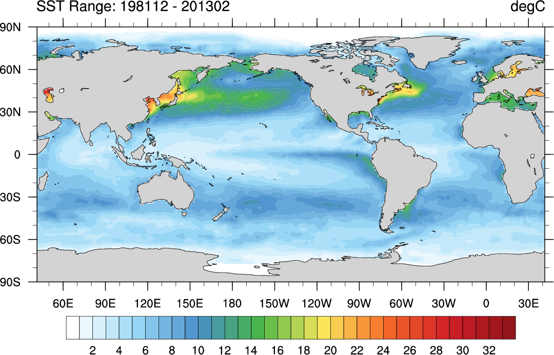
SST range (C) over the period Dec. 1981 - Feb. 2013.
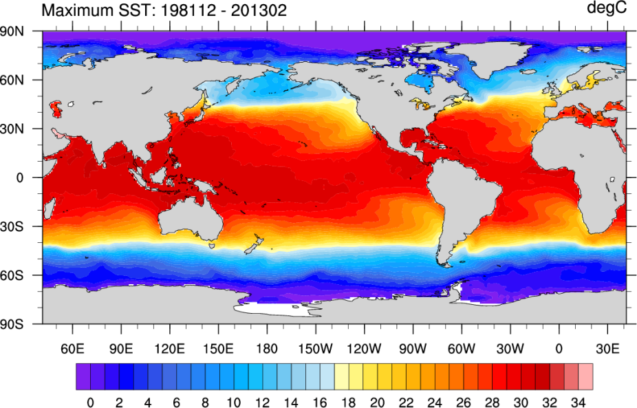
Maximum SST(C) over the period Dec. 1981 - Feb. 2013.
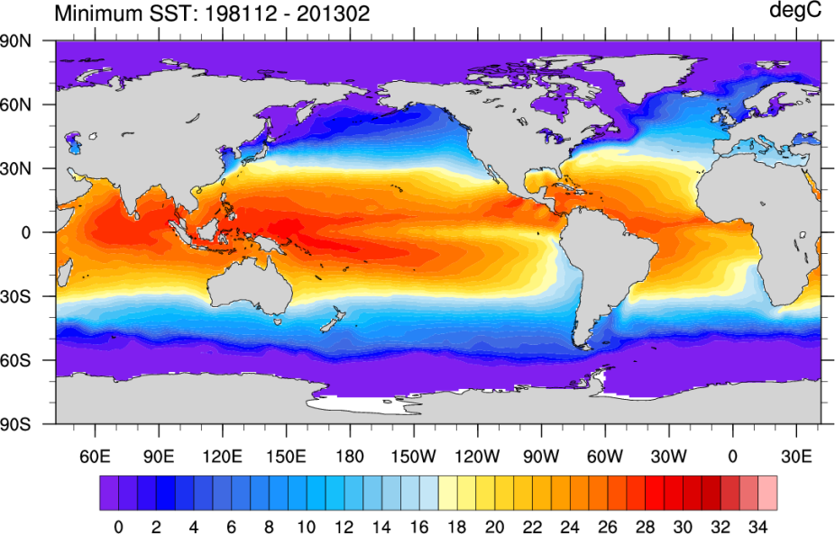
Minimum SST(C) over the period Dec. 1981 - Feb. 2013.
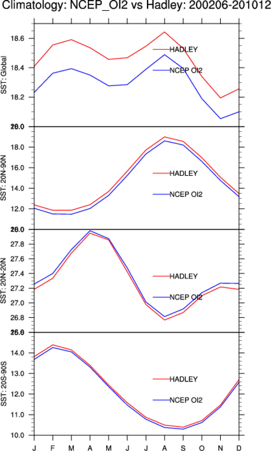
Annual cycle of climatological (200206-201012) areal mean SST: Globe, 20N-90N, 20S-20N, 20S-90S for the NCEP-OI2 and Hadley Centre (HadISST) datasets. The time period was chosen to match the AMSR-E period.
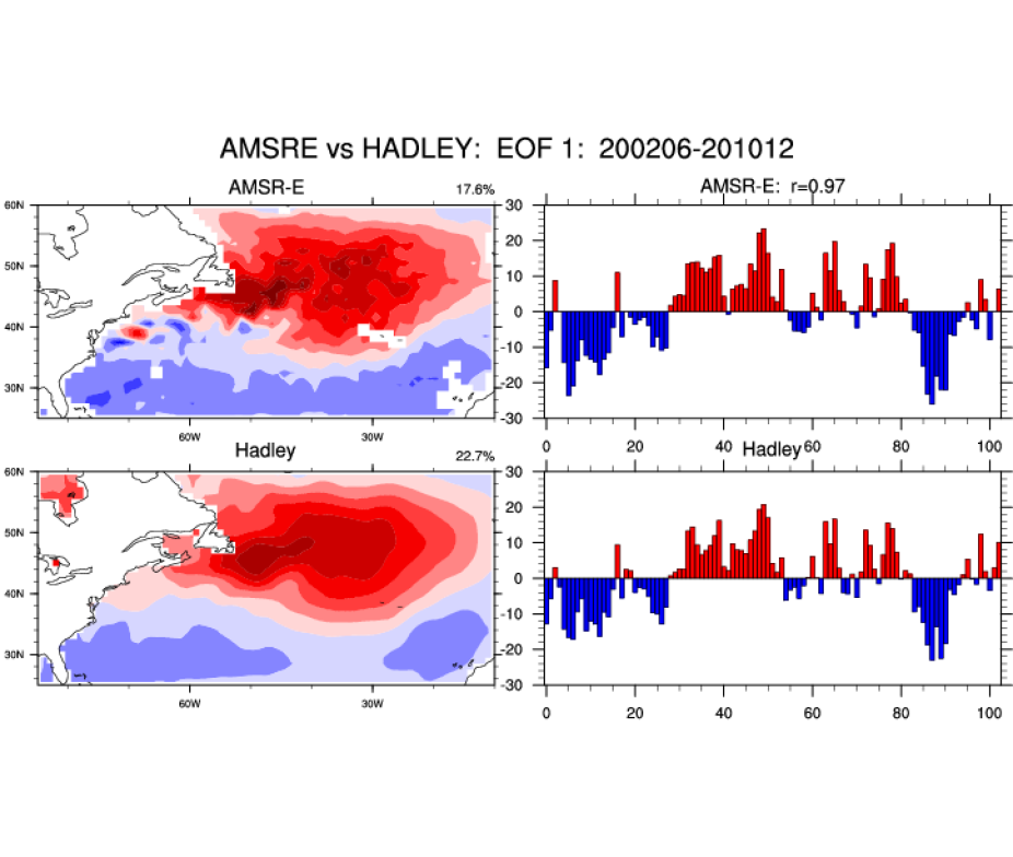
EOF 1 (25N-60N, 275-330E) for the NCEP-OI2 and Hadley Center (HadISST) data sets. The linear correlation coefficient between the principal component time series is 0.98. The time period was chosen to match the AMSR-E period.
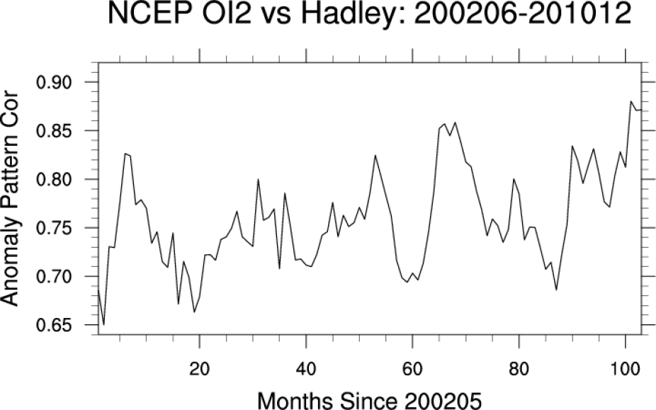
Global anomaly pattern correlations (NCEP-OI2 and Hadley Center) for the period 200206-201012. The time period was chosen to match the AMSR-E period.
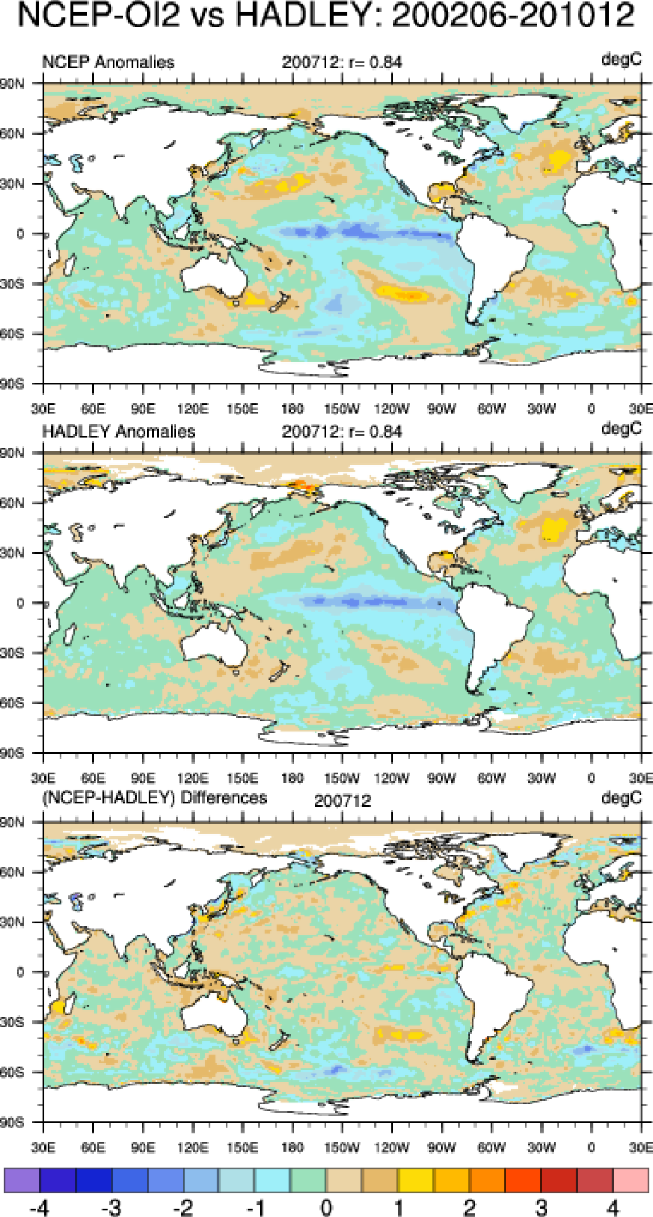
Anomalies between the respective NCEP OI2 and Hadley (HadISST) December climatologies over the period 200206-201012. Top: NCEP (200212)- NCEP; Middle: Hadley (200212)- Hadley. Bottom: Differences between the NCEP and Hadley for 200212. The anomaly pattern correlation between the Top and Middle is 0.82.

Anomalies between the respective NCEP OI2 and Hadley (HadISST) December climatologies over the period 200206-201012. Top: NCEP (200612)- NCEP; Middle: Hadley (200612)- Hadley. Bottom: Differences between the NCEP and Hadley for 200612. The anomaly pattern correlation between the Top and Middle is 0.78.
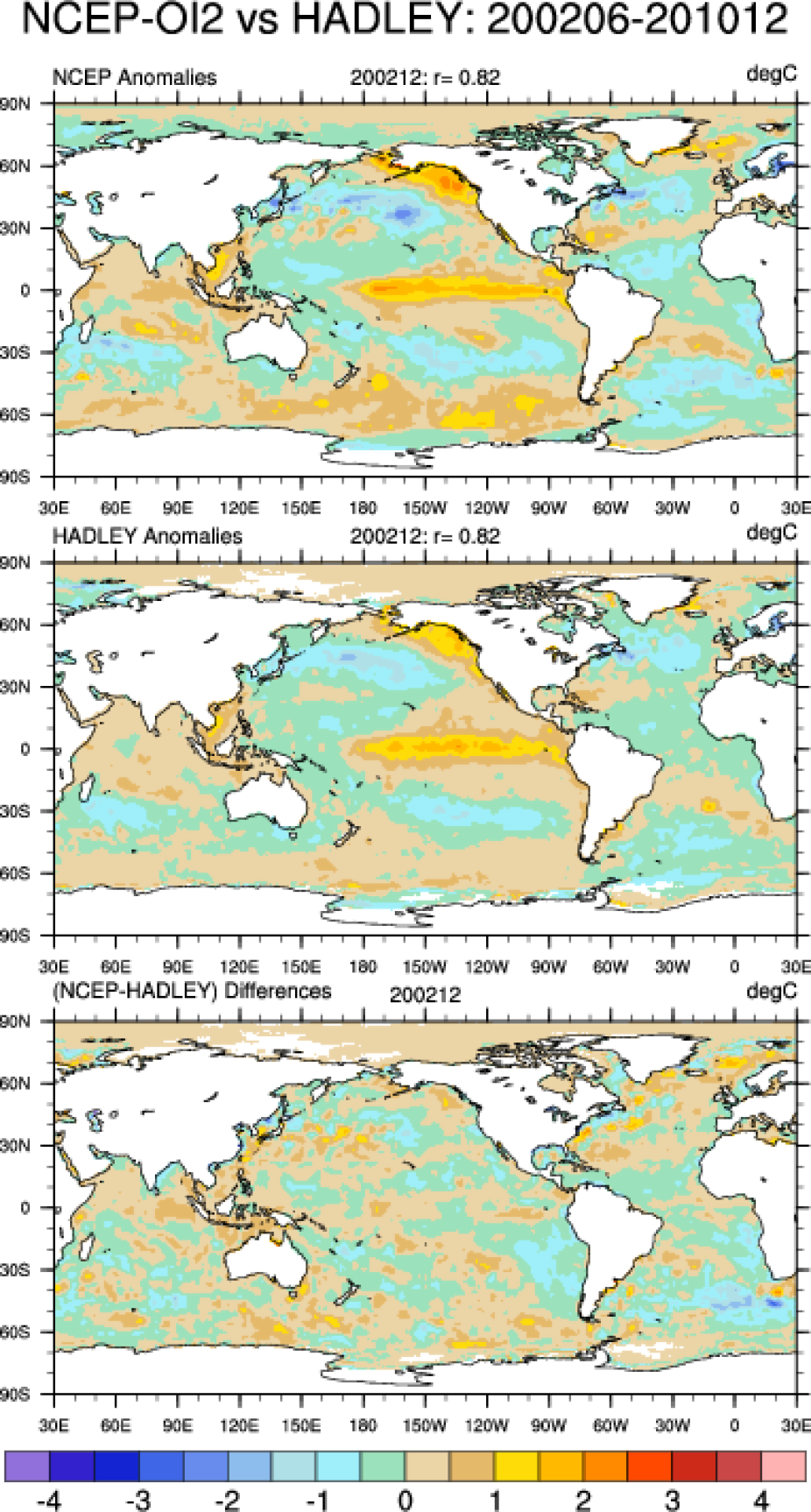
Anomalies between the respective NCEP OI2 and Hadley (HadISST) December climatologies over the period 200206-201012. Top: NCEP (200712)- NCEP; Middle: Hadley (200712)- Hadley. Bottom: Differences between the NCEP and Hadley for 200712. The anomaly pattern
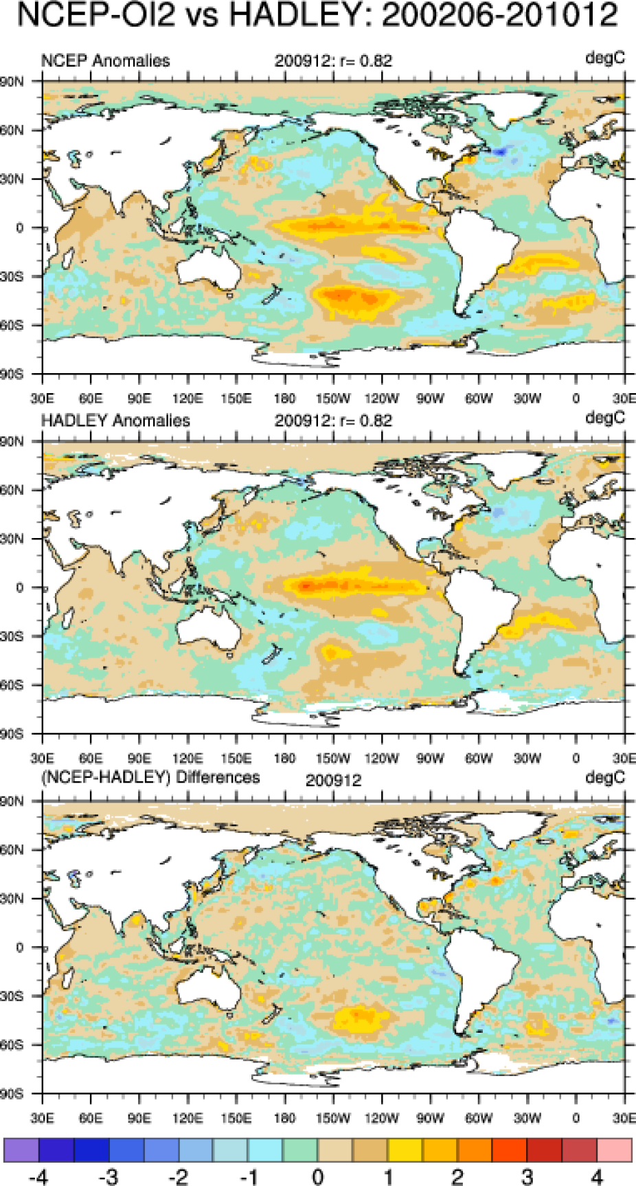
Anomalies between the respective NCEP OI2 and Hadley (HadISST) December climatologies over the period 200206-201012. Top: NCEP (200912)- NCEP; Middle: Hadley (200912)- Hadley. Bottom: Differences between the NCEP and Hadley for 200912. The anomaly pattern correlation between the Top and Middle is 0.82.
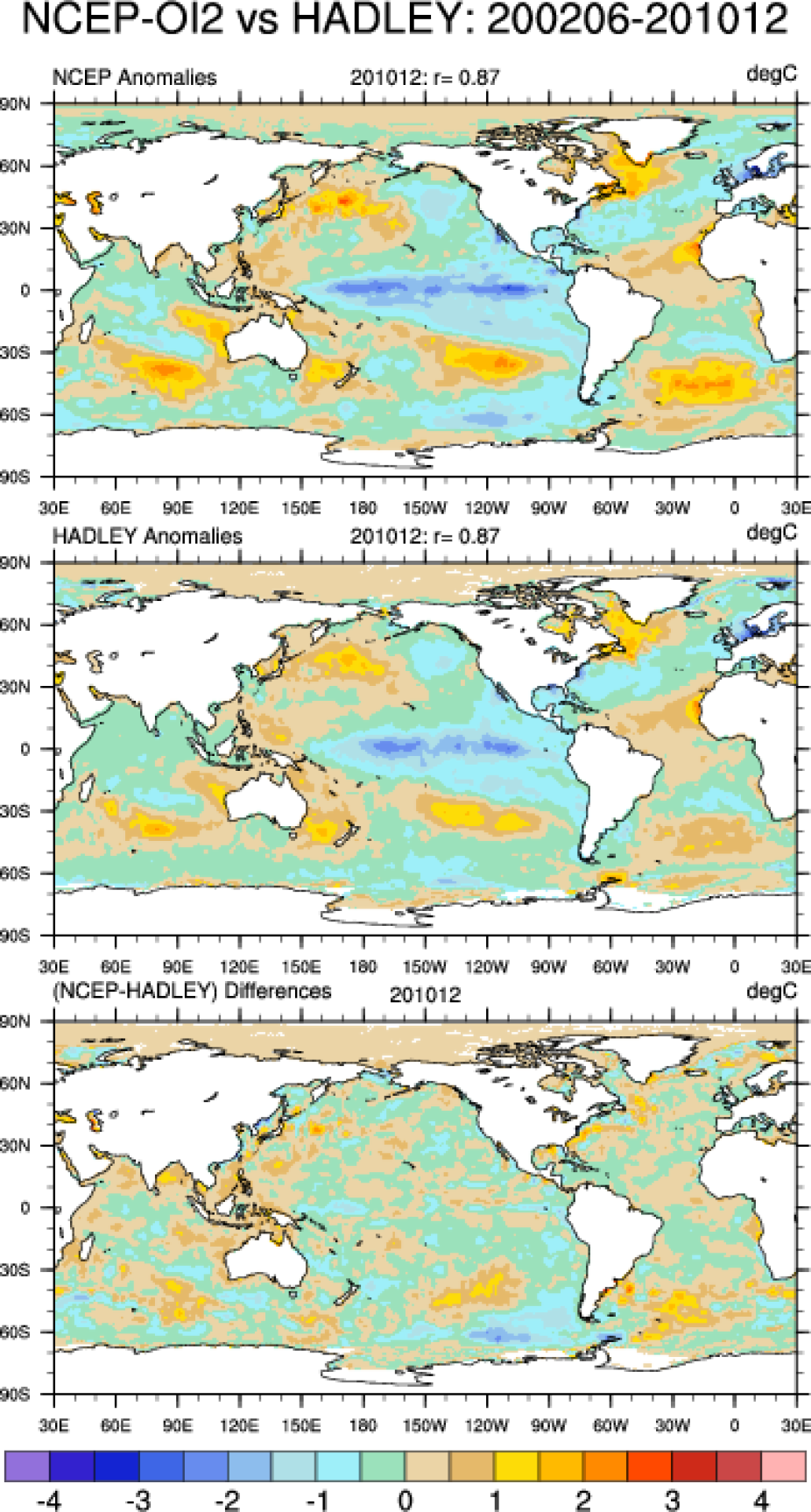
Anomalies between the respective NCEP OI2 and Hadley (HadISST) December climatologies over the period 200206-201012. Top: NCEP (201012)- NCEP; Middle: Hadley (201012)- Hadley. Bottom: Differences between the NCEP and Hadley for 201012. The anomaly pattern correlation between the Top and Middle is 0.87.