Southern Ocean State Estimate (SOSE)
The Southern Ocean State Estimate (SOSE) is a model-generated best fit to Southern Ocean observations. As such, it provides a quantitatively useful climatology of the mean-state of the Southern Ocean. Technically, SOSE is a solution to the MITgcm. SOSE is a gridded dataset at 1/6 ° horizontal resolution, available at timesteps from daily to annually. Observations used include Argo float profiles, shipboard CTD measurements, various mooring data, satellite measurements of sea surface height and sea ice, among others. Caveats about the use of SOSE are broadly similar to issues with reanalyses, in that the SOSE is most reliable in regions and for variables with good observational coverage, and more uncertain in regions and for variables with fewer observational constraints. Misfits to observations can also arise due to errors in the assimilation procedure and model biases. In light of these issues, numerous validations of SOSE have been conducted, and the major biases in SOSE are well documented, as described in the Expert Guidance section of this webpage. For climate model evaluation, SOSE provides advantages over other climatologies such as the World Ocean Atlas by providing a self-consistent state estimate that satisfies momentum, volume, heat and freshwater conservation.
Key Strengths
Key Limitations
Mazloff, Matthew R., Patrick Heimbach, Carl Wunsch, 2010: An Eddy-Permitting Southern Ocean State Estimate. J. Phys. Oceanogr., 40, 880–899.
Expert Developer Guidance
The following was contributed by Matthew Mazloff, September, 2016:
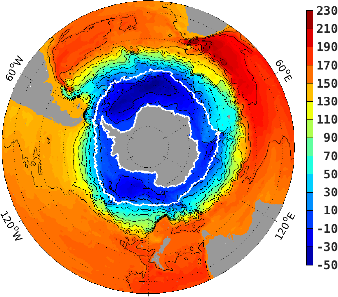
A 2005-2010 Southern Ocean state estimate (SOSE) has been produced and made available (http://sose.ucsd.edu). The mean circulation is shown in Figure 1. It is based on the setup described in Mazloff et al. (2010). The goal of the the SOSE effort it to provide a basis for analyzing the underlying physics controlling the circulation and to provide a quantitatively useful climate baseline. This contribution to the Climate Data Guide is in keeping with the latter goal. SOSE is a dynamically mapped product, and like other mapped products has weaknesses due primarily to model error and lack of constraints. Here we inform use of the state estimate.
The SOSE is a solution to the MITgcm. The model is configured at 1/6 ° resolution and 42 depth levels of varying thickness. It has a sea ice model, and uses the KPP mixed layer parameterization. An atmospheric boundary layer scheme is used to determine fluxes of heat, freshwater (salt), and momentum via bulk formulae (Large and Yeager 2008). What makes SOSE unique is that the initial conditions, the northern boundary condition, and the atmospheric state are solved for via the adjoint method (also known as 4D-Var). The air-sea exchanges produced are constrained to be within a reasonable range, and often correct known biases in the first guess fluxes. For more on the fluxes from SOSE see http://sose.ucsd.edu/TechDocs/SOSE verification example JAN 26 2015o.pdf or Cerovecki et al. (2011).
SOSE constraints come from various sources. In situ measurements include those that were available from the National Oceanographic Data Center (NODC; https://www.nodc.noaa.gov). This included shipboard CTD measurements, instrument-mounted elephant seal profiles (now known as the MEOP program), and Argo float profiles. The CliVar and Carbon Hydrographic Data Office (CCHDO) was also used, and redundancies between this repository and NODC were removed. Expendable bathythermograph (XBT) profiles were obtained from http://www-hrx.ucsd.edu. Process study field program data was also used as a constraint when available. Measurements from these include those taken as part of the Diapycnal and Isopycnal Mixing Experiment in the Southern Ocean (DIMES) project, the mooring array in Drake Passage from the cDrake program, and the shipboard and mooring data in the Amundsen Sea from the Oden expeditions. Measurements from the Antarctic Marine Living Resources Long Term Ecological Research program (AMLR-LTER) were also used. Satellite measurements included sea surface height measurements obtained from the Radar Altimetry Database System (RADS; http://rads.tudelft.nl), optimally interpolated sea surface temperature from microwave radiometers (http://www.remss.com), sea ice concentrations from the National Snow and Ice Data Center (https://nsidc.org). Constraints also included bottom pressure estimates (http://grace.jpl.nasa.gov/data/get-data/ocean-bottom-pressure) and mean dynamic topography obtained from the Technical University of Denmark (http://www.space.dtu.dk/english).
As a mapped product the SOSE output may be easily compared to the ocean state from climate models. To understand the importance of discrepancies, however, requires understanding where SOSE is consistent with observations and where it is problematic. Uncertainty in SOSE arises from lack of constraints and model errors. One can get a feel for both components by looking at the fit to Argo measurements. In regions where no misfit is plotted the solution is likely uncertain due to lack of sufficient constraints. In regions where there is a large misfit to Argo it is likely that errors in the assimilation procedure produced an uncertain SOSE.
Below we answer some “general Climate Data Guide questions."
What are the key limitations of this data set?
The SOSE solution does have some inconsistencies with the observations. With adjoint method optimization it is often most challenging to fit the halocline and thermocline variability, and as a measure of this fit we compare the solution to Argo at 100m. Figure (2) and (3) shows the model is too warm and salty at this depth poleward of 60° S. This implies that the pycnocline is too shallow in the subpolar gyres, consistent with the bias assessment for the Amundsen Sea in Rodriguez et al. (2016). Another significant bias is that the Argentine basin is too cold and fresh. A mean bias is not obvious in the Antarctic Circumpolar Current. At 1,500 m time mean biases are apparent, but far less significant (Fig. 4 and 5). A notable bias is that the Agulhas Retroflection and Subantarctic Front region in the Indian Sector is warmer and fresher than observed.
Upper ocean stratification is assessed here (Figures 6-9) by sampling the model as Argo sampled the true ocean, and then estimating mixed layer depth from those profiles by calculating the depth where the potential density exceeds the surface potential density by 0.3 kg m−3. Though differences are subtle, it is often the case that when observed mixed layers are shallow the SOSE mixed layers are too shallow, and when observed mixed layers are deep the SOSE mixed layers are too deep.
Though not a user-friendly document, http://sose.ucsd.edu/TechDocs/combinedpdf iter100.pdf, does provide more comparisons to in situ constraints and may be useful if there is a specific comparison one wishes to investigate. More examples of validation are given in the next section. Users are also encouraged to contact us to discuss SOSE limitations (contact information at http://sose.ucsd.edu).
What are the key strengths of this data set?
The great benefit of the SOSE solution is that it is a gridded product that obeys model physics and is largely consistent with observations. That it is a model solution makes it accessible to a large user community. As noted directly above, there are some inconsistencies between the SOSE solution and observations. These are, however, documented. Besides the validation above, documentation can be found on http://sose.ucsd.edu and in numerous publications. For example, extensive validation of the surface hydrography and sea ice is in the supplementary material of Abernathey et al. (2016). Extensive validation of the properties and evolution of mode water has been published in Cerovecki and Mazloff (2015) and at http://sose.ucsd.edu/TechDocs/Cerovecki SOSE60 biases.pdf. The mean sea surface height is discussed in Griesel et al. (2012). The velocity structure in Drake Passage is compared to observations in Firing et al. (2011). Assessment of the surface fluxes is available in Cerovecki et al. (2011). Some of these references evaluate older SOSE iterations, but in general the conclusions hold for the most recent published SOSE solution available at http://sose.ucsd.edu/sose state estimation data 05to10.html. Extensive documentation makes it possible to determine the accuracy of SOSE with respect to a certain metric, dataset, or region.
We note that this SOSE setup is no longer under development. Current development is towards the goal of estimating the Southern Ocean carbon cycle as part of the Southern Ocean Carbon and Climate Observations and Modeling project (http://soccom.princeton.edu/). The validation of the solution discussed here does not reflect the biogeochemical SOSE effort. Validation for that effort is being documented at http://sose.ucsd.edu/bsose valid.html
What are the typical research applications of this data set?
SOSE is an estimate of the baseline Southern Ocean state, which may be used to validate climate models. It is also a resource for understanding the Southern Ocean governing dynamics. It has been used, for example, to understand what governs the SO momentum budget (Mazloff et al. 2014; Masich et al. 2015) and heat budget (Tamsitt et al. 2016).
What are the most common mistakes that users encounter when processing or interpreting these data?
There is no “nudging” to the observational constraints in SOSE (i.e. no unphysical sources or sinks in the governing dynamics). Because we have a strong constraint to obey model physics the fronts and eddies are usually not in the right place at the right time. The initial goal of SOSE is to attain consistency with the observed large scale ocean structure.
The resolution and constraints are poor near Antarctica. SOSE has been used to study regions poleward of the ACC, however, one should keep in mind the heightened uncertainty in this region.
What are some comparable data sets?
SOSE is produced by the consortium for Estimating the Circulation and Climate of the Ocean (ECCO; http://ecco-group.org/). Comparable datasets are produced by this group, including a global ocean state estimate for the years 1992 to 2015 (Forget et al. 2015). See http://ecco-group.org/products.htm for a list of ECCO products.
Climatologies (e.g. the World Ocean Atlas) are often used to evaluate climate models, and SOSE may also be used this way. There will be differences between SOSE and climatologies due to discrepancies in the way the products were derived and the constraints used. No mapping method is truly optimal. Weaknesses in SOSE with respect to climatologies include the fact that SOSE is more likely to introduce biases and drifts due to numerical model errors. Climatologies have errors due to assumptions in the prescribed spatial correlation scales and a poor accounting for temporal correlations. As observational density increases objectively mapped products can better account for temporal information, and we are now seeing this with the Argo objectively mapped product (http://sio-argo.ucsd.edu/RG Climatology.html). Nevertheless, these climatologies only map temperature and salinity and do not propagate information between other components of the system. An advantage of the SOSE resource is that it provides a self-consistent mapped state, with stable stratification and velocities that satisfy momentum conservation.
How is uncertainty characterized in these data?
A formal uncertainty map is not provided. One can gauge uncertainty as discussed above in the section on “key limitations”
Were corrections made to account for changes in observing systems or practices, sampling density, satellite drift, or similar issues?
The time period of the optimization, 2005–2010, is one where the Southern Ocean observing system was rather stable. It was not necessary to account for any changes in the the observing system. Though the optimization procedure for 2005-2007 was different than 2008-2010, we do not believe it led to a change in the consistency with observations in these two periods.
How do I best compare these data with model output?
As the SOSE is model output, it is rather straightforward to compare to other model solutions. SOSE is on a C-grid at 1/6 ° resolution and interpolation is likely necessary. SOSE is available as daily, 5-day, monthly, and annual averages at http://sose.ucsd.edu/sose stateestimation data 05to10.html. SOSE uses partial cells; for integrated calculations (e.g. transport) one should use the appropriate cell height fractions. Please contact us if you have any questions (contact information at http://sose.ucsd.edu).
Are there spurious (non-climatic) features in the temporal record?
There should be no spurious (non-climatic) features in the temporal record. There is, however, a known adiabatic drift in the circumpolar deep water classes in the Pacific Sector. This drift is discussed in Cerovecki and Mazloff (2015).
Acknowledgments
SOSE was produced by the ECCO consortium with support from several NASA and NSF grants. Computational resourced were provided by the Extreme Science and Engineering Discovery Environment (XSEDE), which is supported by NSF grant number MCA06N007. We are grateful to the very large group of oceanographers who collected and processed the observations used here; without whom none of this would be possible.
When using the SOSE solution please reference Mazloff et al. (2010). ##
Cite this page
Acknowledgement of any material taken from or knowledge gained from this page is appreciated:
Mazloff, Matthew & National Center for Atmospheric Research Staff (Eds). Last modified "The Climate Data Guide: Southern Ocean State Estimate (SOSE).” Retrieved from https://climatedataguide.ucar.edu/climate-data/southern-ocean-state-estimate-sose on 2026-02-27.
Citation of datasets is separate and should be done according to the data providers' instructions. If known to us, data citation instructions are given in the Data Access section, above.
Acknowledgement of the Climate Data Guide project is also appreciated:
Schneider, D. P., C. Deser, J. Fasullo, and K. E. Trenberth, 2013: Climate Data Guide Spurs Discovery and Understanding. Eos Trans. AGU, 94, 121–122, https://doi.org/10.1002/2013eo130001
Key Figures

Figure 1. The time-mean vertically integrated streamfunction in Sverdrups. The maximum seaice extent is denoted with the thick white line. (contributed by M Mazloff)
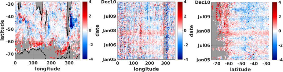
Figure 2 Mean binned potential temperature misfit (SOSE minus Argo) at 100m in °C. Left is time mean, center is meridional mean, and right is zonal mean. (contributed by M Mazloff)
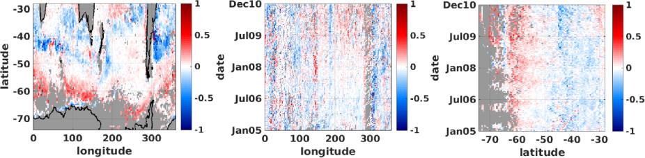
Figure 3 Mean binned salinity misfit (SOSE minus Argo) at 100m in psu. Left is time mean, center is meridional mean, and right is zonal mean. (contributed by M Mazloff)
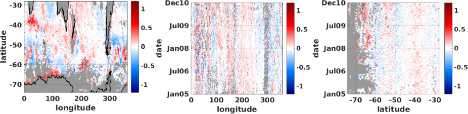
Figure 4 Mean binned potential temperature misfit (SOSE minus Argo) at 1500m in °C. Left is time mean, center is meridional mean, and right is zonal mean. (contributed by M Mazloff)
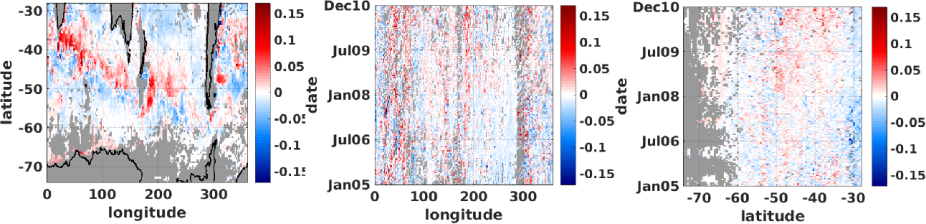
Figure 5 Mean binned salinity misfit (SOSE minus Argo) at 1500m in psu. Left is time mean, center is meridional mean, and right is zonal mean. (contributed by M Mazloff)
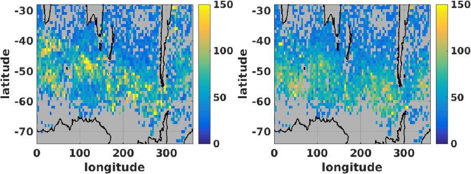
Figure 6 December–January–February bin average mixed layer depth (m). Mixed layer depth estimated as the depth where the potential density exceeds the surface potential density by 0.3 kg m-3. Left is from SOSE sampled as Argo floats sampled the ocean and right is from Argo profiles. (contributed by M Mazloff)
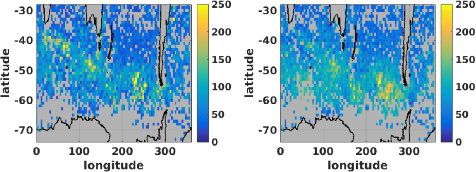
Figure 7 March–April–May bin average mixed layer depth (m). Mixed layer depth estimated as the depth where the potential density exceeds the surface potential density by 0.3 kg m-3. Left is from SOSE sampled as Argo floats sampled the ocean and right is from Argo profiles. (contributed by M Mazloff)
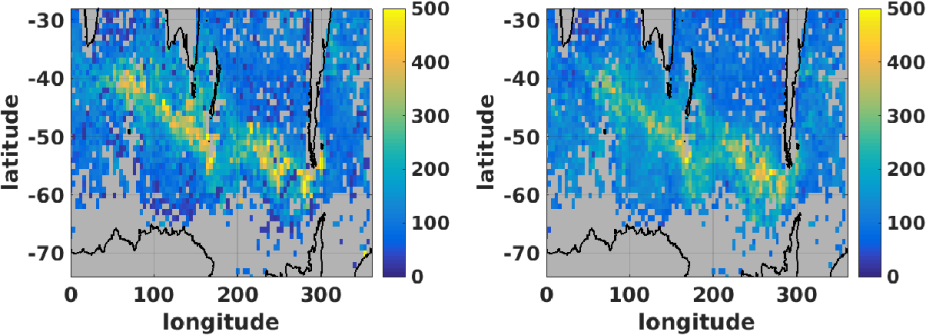
Figure 8 June–July–Aug bin average mixed layer depth (m). Mixed layer depth estimated as the depth where the potential density exceeds the surface potential density by 0.3 kg m-3 Left is from SOSE sampled as Argo floats sampled the ocean and right is from Argo profiles. (contributed by M Mazloff)
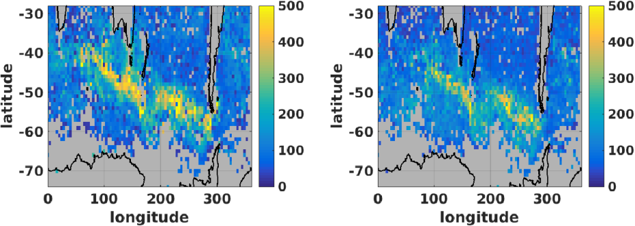
Figure 9 September–October–November bin average mixed layer depth (m). Mixed layer depth estimated as the depth where the potential density exceeds the surface potential density by 0.3 kg m-3. Left is from SOSE sampled as Argo floats sampled the ocean and right is from Argo profiles. (contributed by M Mazloff)