Standardized Precipitation Evapotranspiration Index (SPEI)
The Standardized Precipitation Evapotranspiration Index (SPEI) is an extension of the widely used Standardized Precipitation Index (SPI). The SPEI is designed to take into account both precipitation and potential evapotranspiration (PET) in determining drought. Thus, unlike the SPI, the SPEI captures the main impact of increased temperatures on water demand. Like the SPI, the SPEI can be calculated on a range of timescales from 1-48 months. At longer timescales (>~18 months), the SPEI has been shown to correlate with the self-calibrating PDSI (sc-PDSI). If only limited data are available, say temperature and precipitation, PET can be estimated with the simple Thornthwaite method. In this simplified approach, variables that can affect PET such as wind speed, surface humidity and solar radiation are not accounted for. In cases where more data are available, a more sophisticated method to calculate PET is often preferred in order to make a more complete accounting of drought variability. However, these additional variables can have large uncertainties.
A gridded SPEI data set is available for 1901-2011 based on CRU TS3.2 input data and the Penman-Monteith method. A real-time SPEI is published for global drought monitoring based on the Thornnthwaite method. Finally, an R package is available for calculating the SPEI from user-selected input data using either the Thornthwaite, Penman-Monteith, or Hargreaves methods.
Key Strengths
Combines multi-timescales aspects of the Standardized Precipitation Index (SPI) with information about evapotranspiration, making it more useful for studies of long-term trends
Statistically based index that requires only climatological information without assumptions about the characteristics of the underlying system
Key Limitations
More data requirements than the precipitation SPI
Sensitive to the method to calculate potential evapotranspiration (PET)
As with other drought indices, a long base period (30-50+ years) that samples the natural variability should be used
Expert Developer Guidance
The following was contributed by Dr. Sergio M. Vicente-Serrano (Instituto Pirenaico de Ecología, Spanish National Research Council), March, 2014:
The World Meteorological Organization (WMO) has adopted the standardized precipitation index (SPI) to be used by national meteorological and hydrological services worldwide to characterize meteorological droughts (Hayes et al., 2011). The WMO provides standard guidelines and software to calculate the SPI (WMO, 2012). Nevertheless, the SPI is based solely on precipitation data, not considering other variables that also determine drought conditions such as temperature, relative humidity, evapotranspiration, wind speed, etc. Thus, the SPI relies on two assumptions: (i) the variability of precipitation is much higher than that of other variables (e.g., the evaporative demand of the atmosphere); and (ii) the other variables are stationary (i.e., they have no temporal trend). The importance of variables other than precipitation is negligible in this framework, and droughts are assumed to be mainly controlled by the temporal variability of precipitation
Given the global temperature increase during the last 150 years and that Earth system models predict a marked increase during the 21st century, it can be expected that temperature rise will have dramatic consequences for drought conditions. Therefore, the use of drought indices that include temperature data in their formulation, such as the palmer drought severity index (PDSI), seems to be preferable than using indices without temperature information to identify warming-related drought impacts on different ecological, hydrological, and agricultural systems. However, the PDSI lacks the multiscalar character of the SPI, essential for assessing drought in relation to different hydrological systems and also for differentiating among different drought types.
It is commonly accepted that drought is a multi-scalar phenomenon since the time period from the arrival of water inputs to availability of a given usable resource differs considerably. Thus, the time scale over which water deficits accumulate becomes extremely important, and functionally separates hydrological, environmental, agricultural and other droughts. For this reason, drought indices must be associated with a specific timescale to be useful for monitoring and management of different usable water resources.
To overcome these limitations, the standardized precipitation evapotranspiration index (SPEI) was recently developed, which combines the sensitivity of PDSI to changes in evaporation demand caused by temperature with the multi-temporal nature of the SPI. The standardized precipitation evapotranspiration index (SPEI) was first proposed by Vicente-Serrano et al. (2010a) as an improved drought index that is especially suited for studies of the effect of global warming on drought severity. Like the PDSI, the SPEI considers the effect of reference evapotranspiration on drought severity, but the multi-scalar nature of the SPEI enables identification of different drought types and drought impacts on diverse systems (Vicente-Serrano et al., 2012, 2013). Thus, the SPEI has the sensitivity of the PDSI in measurement of evaporative demand of the atmosphere (caused by fluctuations and trends in climatic variables other than precipitation), is simple to calculate, and is multi-scalar, like the standardized precipitation index (SPI). Vicente-Serrano et al. (2010a, 2010b, 2011, 2012) and Beguería et al. (2014) have provided complete descriptions of the theory behind the SPEI, computational details, and comparisons with other popular drought indicators such as the PDSI and the SPI.
The procedure for calculating the SPEI is similar to that for the SPI. However, the SPEI uses the difference between precipitation and reference evapotranspiration (P – ETo), rather than precipitation (P) as the input. The climatic water balance compares the available water (P) with the atmospheric evaporative demand (ETo), and therefore provides a more reliable measure of drought severity than only considering precipitation. The ETo is the evapotranspiration rate of a reference surface (a well-watered hypothetical grass reference crop with specific characteristics). In the Food and Agricultural Organization (FAO) manual to calculate ETo, Allen et al. (1998) stressed that ETo represents “the evaporative demand of the atmosphere independently of crop type, crop development and management practices. [ . . . ] The only factors affecting ETo are climatic parameters. Consequently, ETo is a climatic parameter, it can be computed from weather data, and it expresses the evaporating power of the atmosphere at a specific location and time of the year”. As a consequence, ETo calculated at different locations or in different seasons are totally comparable. This is different to the concept of actual evaporation (ETa), which is the water lost under real conditions (i.e. considering the water available in the soils, the vegetation or crop type and state, physiological mechanisms, climate, etc).
The idea behind the SPEI is to compare the highest possible evapotranspiration (what we call the evaporative demand by the atmosphere) with the current water availability. Thus, precipitation (accumulated over a period of time) in the SPEI stands for the water availability, while ETo stands for the atmospheric water demand. ETa would be a poor estimator of this demand, since it depends in turn on the current water availability. On the other hand, the very definition of ETo indicates that it refers to the maximum amount of water that would be transferred to the atmosphere by the soils and vegetation if there were no water supply deficit. Using ETo as an estimator of the true evaporative demand seems, thus, a more convenient choice. ETa is a poor indicator of drought stress, albeit the difference between input Precipitation (P) and demand (ETo). In fact, using the ETa in the SPEI would make sense as a replacement of P. Indeed, the ETa could be a better estimator than P of the amount of water actually used by the vegetation, hence the balance ETa – ETo would provide a better indicator of the stress (or no stress) that the system is undergoing in any given moment. ETa is not used in the SPEI, and P is used instead as an estimator of water available to the system because of the difficulties involved in estimating ETa. The ETa is not only determined by the precipitation input and the evapotranspiration demand but also by the water balance of the soil and plants, which depends on soil and vegetation parameters that are difficult to estimate and are not stationary in time. Complex physically based models are normally required in order to estimate ETa for a given system, and then there are specific models for each system under consideration (tree and forest growth models, crop models, soil hydrology models, catchment hydrology models, etc). The SPEI was developed as a generalist drought index susceptible of being applied to a large variety of systems, so depending on a particular model was not an option. Thus, the precipitation accumulated over an arbitrary period of time that could be adapted to the behaviour shown by a given system, can be considered a convenient approximation to the amount of water available to a system in any given moment (See further discussion on ETo and ETa issues in Vicente-Serrano et al., 2011 and Beguería et al., 2014).
SPEI uses a climatic water balance (Di = Pi-ETo) obtained at various time scales (k) (i.e. over one month, two months, three months, etc.). For example, to obtain the 6-month SPEI, first a time series is constructed by the sum of D values from five months before to the current month. Given the strong seasonal differences in the magnitude of P and ETo and the climate regimes of each site, to obtain SPEI series comparable in space and time, it is necessary to transform the D series using equal probability to a normal distribution with a mean of zero and standard deviation of one so the values of the SPEI are really in standard deviations and lacks of seasonal effects.
For this purpose, D values are fit to a probability distribution to transform the original values to standardized units that are comparable in space and time and at different SPEI time scales, following the same procedure as that for the SPI. Different analysis suggested selection of the Log-logistic distribution for standardizing the D series to obtain the SPEI (Vicente-Serrano et al., 2010a) since the Log-logistic distribution adapted very well to the Dseries for all time scales and climate regions. With very few exceptions, for most regions worldwide a good fit was found between the log-logistic distribution and Dk series, independent of the time scale (k) and the month of the year (Vicente-Serrano et al., 2010b). This guarantees the robustness of SPEI calculations based on such probability distribution.
The probability density function of a three parameter Log-logistic distributed variable is expressed as:
where α, β and γ are scale, shape and origin parameters, respectively, for D values in the range (γ> D <∞ ).
Parameters of the Log-logistic distribution can be obtained following different procedures. Among them, the Probability-weighted moments (PWMs) procedure is a robust and easy approach. The PWMs of order s are calculated as:
![]()
where Fi is a plotting position estimator calculated following:
![]()
where i is the range of observations arranged in increasing order, and N is the number of data points.
When PWMs are calculated, the parameters of the Log-logistic distribution can be obtained following:
![]()
![]()
![]()
where Γ(Β ) is the gamma function of Β.
The probability distribution function of the D series according to the Log-logistic distribution is given by:
![]()
With F(x) the SPEI can easily be obtained as the standardized values of F(x):
![]()
where
![]() for P ≤ 0.5
for P ≤ 0.5
and P is the probability of exceeding a determined D value, P =1-F(x). If P > 0.5, P is replaced by 1-P and the sign of the resultant SPEI is reversed. The constants are: C0 = 2.515517, C1 = 0.802853, C2 = 0.010328, d1 = 1.432788, d2 = 0.189269, d3 = 0.001308. The average value of SPEI is 0, and the standard deviation is 1. The SPEI is a standardized variable, and it can therefore be compared with other SPEI values over time and space. An SPEI of 0 indicates a value corresponding to 50% of the cumulative probability of D, according to a Log-logistic distribution.
Estimation of the log-logistic parameters is important because spatial and temporal comparability of drought indices is important for accurate drought analysis and monitoring. It is necessary that SPEI series at different sites have the same average (x =0) and Standard Deviation (SD=1); the same is applicable to series of the SPEI recorded at the same location but at different timescales. Parameter estimation can lead to bias and errors in variance, so the method used for estimation is very important. Originally the probability weighted moments (PWMs) based on the plotting position formula (Fi) was proposed to calculate SPEI (Vicente-Serrano et al., 2010a), but Beguería et al. (2014) have showed that the plotting position estimator was not an optimal method for computation of SPEI, because it led to biased SDs. Moreover, the SD increased with increasing SPEI time scale, so that SPEI series at different time scales cannot be compared for a given site. Moreover, the plotting position method led to many cases with no solution (more than 2% in some areas of the world), and the number of such cases increased as the time scale decreased. For these reasons an unbiased PWM estimator was proposed for SPEI calculation. The unbiased PWM estimator is obtained according to
The unbiased PWM method did not lead to unsuccessful fits to a log-logistic distribution, provided stationary SDs among space and SPEI time-scales and provided a solution for any D value (with a few exceptions).
The original formulation of the SPEI suggested use of the Thornthwaite equation for estimation of ETo (Thornthwaite, 1948). This equation only requires mean daily temperature and latitude of the site, and it was used due to limited data availability. Nevertheless, the use of a particular equation for estimation of ETo is not central for the calculation of SPEI, and other equations can also be used. The more robust FAO-56 Penman-Monteith equation (Allen et al., 1998) is recommended if data is available (relative humidity, temperature, wind speed and solar radiation). If the data needed for this equation are not available, the Hargreaves equation (first) or the Thornthwaite equation (second) are recommended. Differences between the SPEI series calculated using the different ETo equations can be significant in some regions of the world. In general, these differences were larger in semi-arid to mesic areas, and smaller in humid regions (Beguería et al., 2014).
In general, the low data requirements of the SPEI, the facility and flexibility of its calculation, and the consideration of the two main elements that determine drought severity (precipitation and atmospheric evaporative demand) are solid reasons to recommend its use over other drought indices. The SPEI can account for the possible effects of temperature variability and temperature extremes beyond the context of global warming. Therefore, given the minor additional data requirements of the SPEI relative to the SPI, use of the former is preferable for the identification, analysis and monitoring of droughts in any climate region of the world. The SPEI fulfills the requirements of a drought index, since its multi-scalar character enables it to be used by different scientific disciplines to detect, monitor and analyze droughts. Like the PDSI and the SPI, the SPEI can measure drought severity according to its intensity and duration, and can identify the onset and end of drought episodes. The SPEI allows comparison of drought severity through time and space, since it can be calculated over a wide range of climates. Keyantash and Dracup (2002) indicated that drought indices must be statistically robust and easily calculated, and have a clear and comprehensible calculation procedure. All these requirements are met by the SPEI. However, a crucial advantage of the SPEI over the most widely used drought indices that consider the effect of ETo on drought severity is that its multi-scalar characteristics enable identification of different drought types and impacts in the context of global warming.
Moreover, the SPEI is purely statistical; it is not intended to reproduce the water balance of any particular system. From this point of view, the advantages of SPEI (and also SPI) regarding other indices are that: i) their calculation only requires climatological information, which is often available and of reasonable quality; ii) they do not require any assumptions about the system being modeled; and iii) they compute the climatological anomalies for periods of exact length (termed the ‘time scale’ of the index). The fact that SPEI is not physically based is more liberating than constraining. The SPI and the SPEI maintain units with a robust statistical meaning, and the series of the various time scales are comparable between them. Moreover, SPI and SPEI have the advantage of determining exactly the period (time scale) in which the antecedent conditions are affecting the value of the index. In addition, the SPI and SPEI are not obtained using smoothing approaches, but by cumulative antecedent climate conditions. Thus, calculation of the time series of a drought index obtained at a given time scale is completely independent of the time series of the index obtained at a different time scale. In addition, the magnitude of the index has a clear statistical meaning, as it is expressed as a standardized anomaly. As the SPI, the SPEI is perfectly comparable in time and space, and across different time-scales, as it corresponds to a standard normal variable. Thus, the same SPEI values occur with the same frequency in all regions of the world, independent of the climate characteristics of the region.
Calculation of the SPEI is implemented in the R package SPEI (http://cran.r-project.org/web/packages/SPEI). This package is preferred over previous implementation in C language (http://digital.csic.es/handle/10261/10002). This latter implementation only allows computation of the original formulation of the SPEI (based on the Thornthwaite ETo equation). The SPEI R package allows three ETo equations (Thornthwaite, Hargreaves and FAO-56 Penman-Monteith). In addition, there are different options for the FAO-56 Penman-Monteith equation, depending on data availability. For example, if data on solar radiation is rarely available, the code can estimate it from the duration of bright sunshine or from the percent cloud cover. Similarly, if data on saturation water pressure is not available, the code can estimate it from the dewpoint temperature, relative humidity, or minimum temperature, sorted from least to most uncertain method.
A gridded SPEI dataset is available at time scales of 1 to 48 months, spatial resolution of 0.5◦ lat/lon, and temporal coverage from January 1901 to December 2011 by use of the Climate Research Unit (CRU TS3.2) (see further details at http://sac.csic.es/spei/database.html). The SPEIbase v.2.2 is available from http://digital.csic.es/handle/10261/72264 in netCDF format, and individual files corresponding to each 0.5◦ grid are available from http://sac.csic.es/spei/database.html.
A global real-time drought monitoring system based on the SPEI is also available at http://sac.csic.es/spei/map/maps.html. This system provides global SPEI maps for the entire earth at a spatial resolution of 0.5◦. The SPEI products are obtained using the Thornthwaite equation for calculation of ETo because necessary global information for calculation of ETo by the FAO-56 Penman-Monteith or Hargreaves equations at real-time are not available. The SPEI global drought monitor provides SPEI time-scales of 1–48 months, allows graphical display of the change in SPEI over time at user-defined sites, and allows downloading of time series of the SPEI at specific points, areas, or the complete dataset in netCDF format. This dataset is different than the SPEIbase v.2.2 dataset, and may be less accurate because climate inputs of the CRU TS3.2 dataset (from which the SPEIbase v.2.2 is computed) undergo careful quality-control, are homogenized, cover a longer time period (1901–2011), and allow calculation of ETo by the more robust FAO-56 Penman-Monteith equation. The main advantage of the drought monitoring system is the near-real time availability of data, which may be important for certain uses. ###
Cite this page
Acknowledgement of any material taken from or knowledge gained from this page is appreciated:
Vicente-Serrano, Sergio M. & National Center for Atmospheric Research Staff (Eds). Last modified "The Climate Data Guide: Standardized Precipitation Evapotranspiration Index (SPEI).” Retrieved from https://climatedataguide.ucar.edu/climate-data/standardized-precipitation-evapotranspiration-index-spei on 2026-02-27.
Citation of datasets is separate and should be done according to the data providers' instructions. If known to us, data citation instructions are given in the Data Access section, above.
Acknowledgement of the Climate Data Guide project is also appreciated:
Schneider, D. P., C. Deser, J. Fasullo, and K. E. Trenberth, 2013: Climate Data Guide Spurs Discovery and Understanding. Eos Trans. AGU, 94, 121–122, https://doi.org/10.1002/2013eo130001
Key Figures

Spatial distribution of 3-month SPEI values in August 2003 from the SPEI Global Drought Monitor (http://sac.csic.es/spei/map/maps.html). Evolution of the 3-month SPI, SPEI and Standardized P-ETa in central France (47ºN-2ºE). Details for the 2003 drought are showed for the three indices. (Contributed by S. Vicente-Serrano)

Magnitude of temporal trends of SPEI series from 1950 to 2009 (SPEI units per decade) for various time scales in grid cells of the global dataset. The scatterplots show the relationship of the magnitude of change for different SPEI models; the solid black line indicates perfect agreement (1:1) and the dashed line indicates a linear fit to the data. (Contributed by S. Vicente-Serrano)
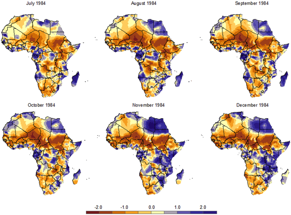
Spatial distribution of the 6-month SPEI for the entire Africa between July and December 1984. (Contributed by S. Vicente-Serrano)
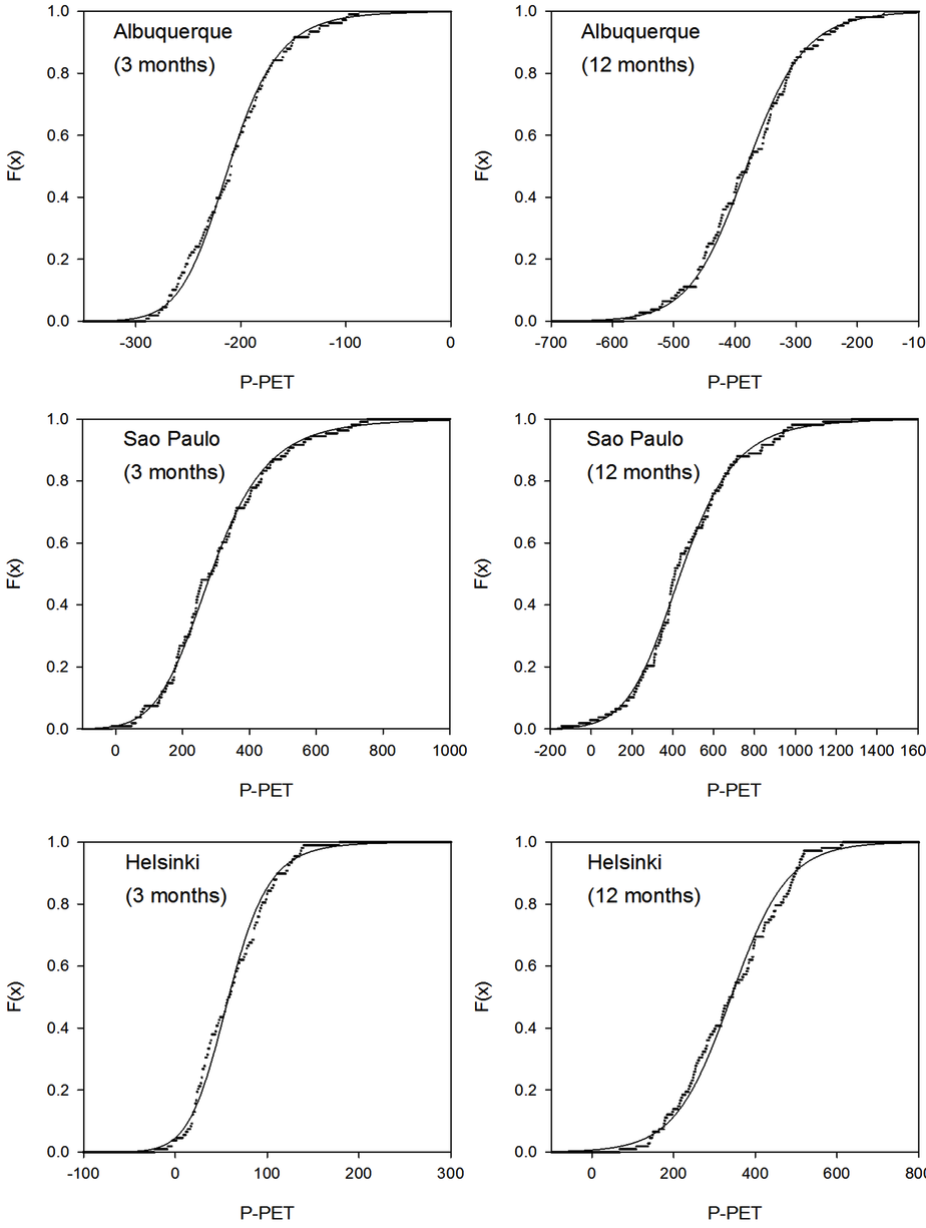
Theoretical according the Log-logistic distribution (black line) vs. empirical (dots) F(x) values for D series at time scales of 3 and 12 months for the observatories at Albuquerque, Sao Paulo and Helsinki. (Contributed by S. Vicente-Serrano)
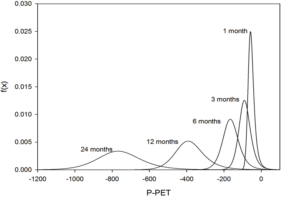
Probability density functions of the Log-logistic distribution for D series calculated at different time scales at the Albuquerque (New Mexico, USA) observatory. (Contributed by S. Vicente-Serrano)
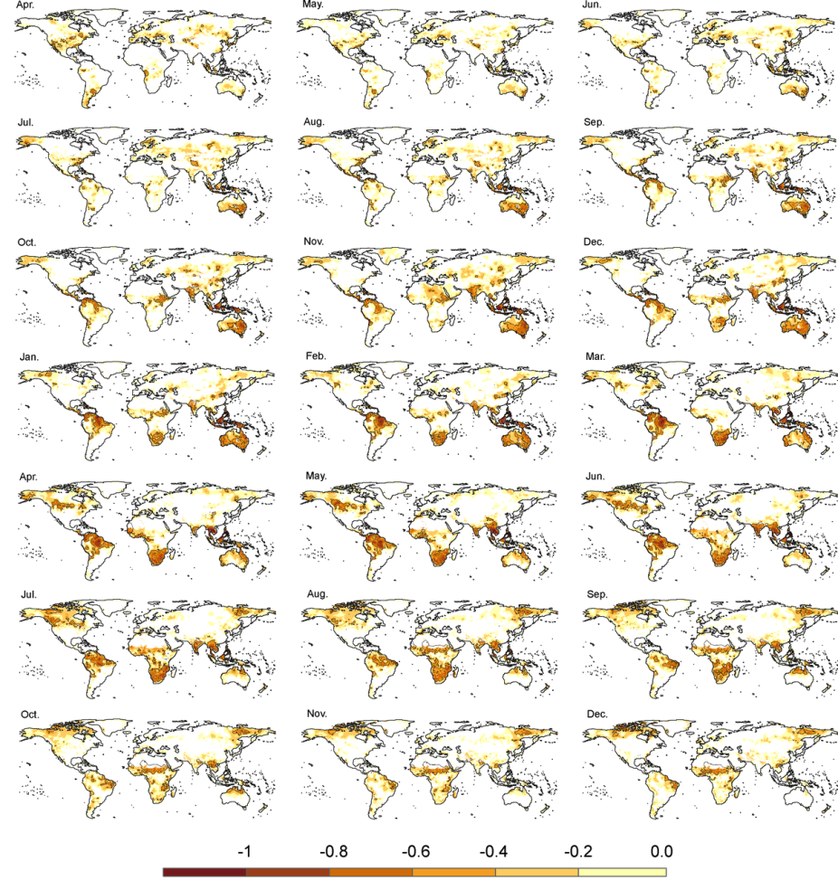
Spatial distribution of the average 12-month SPEI composite anomalies during El Niño years and the years preceding. Orange/reds identify areas in which significant differences in the SPEI average were found between the El Niño years and other years. Grays identify negative but non-significant anomalies. (Contributed by S. Vicente-Serrano)
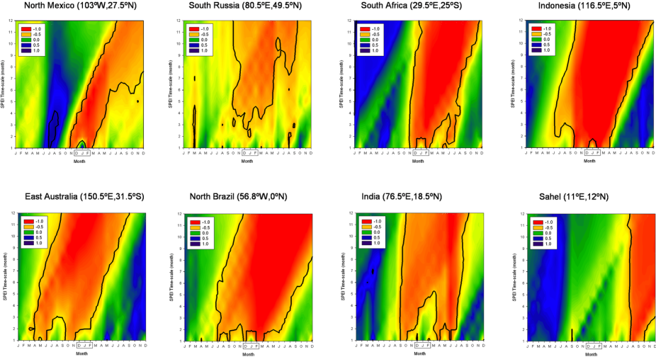
Average SPEI values at the time scales of 1−12 months in eight representative regions of the world during the ENSO phases that drive drought conditions in each region: i) La Niña (northern Mexico and southern Russia), and ii) El Niño (South Africa, Indonesia, eastern Australia, northern Brazil, India and the Sahel). The black lines identify months and time scales when significant differences in the SPEI averages were found between the corresponding ENSO phase and the remaining years. (Contributed by S. Vicente-Serrano)

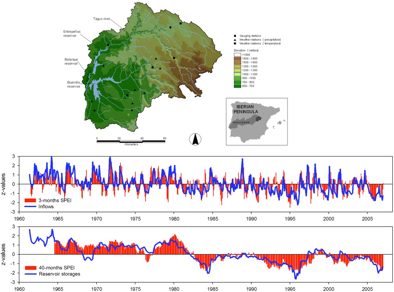
Evolution of hydrological drought index and SPEI in the headwaters of the Tagus basin (central Spain). (Contributed by S. Vicente-Serrano)
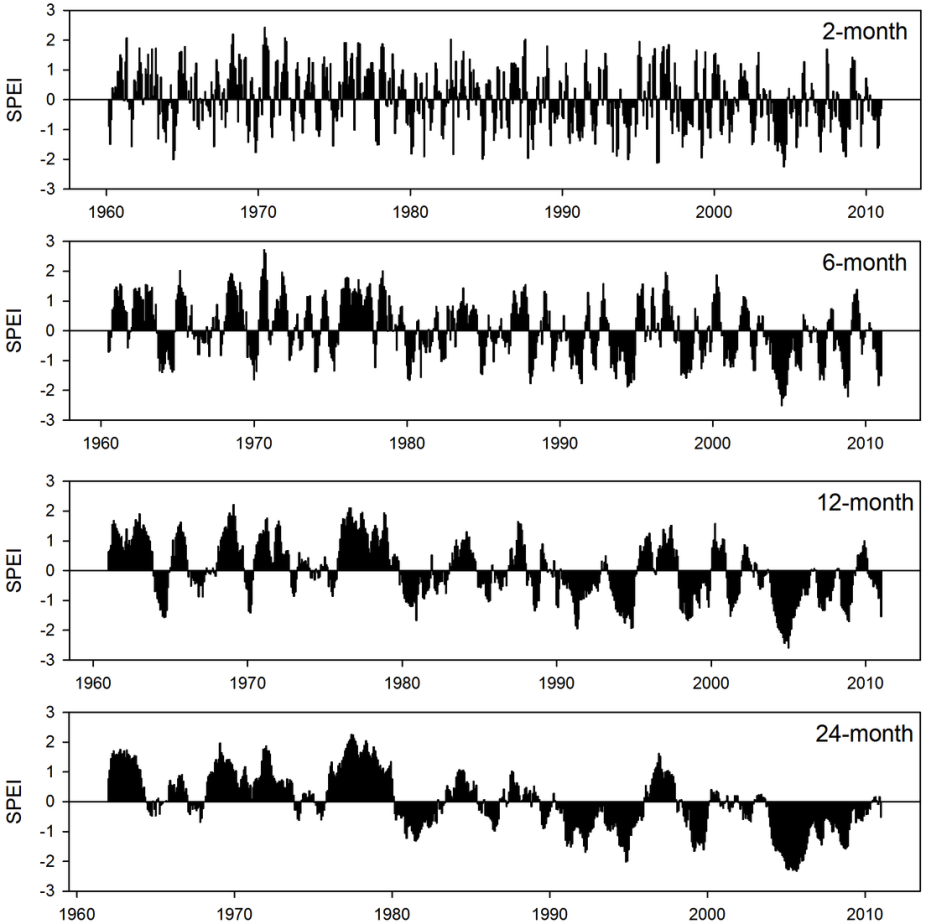
Evolution of the SPEI at various time scales for the entire Iberian Peninsula. (Contributed by S. Vicente-Serrano).
Other Information
- Allen, R.G., Pereira, L.S., Raes, D. and Smith, M., (1998) - Crop evapotranspiration - Guidelines for computing crop water requirements - FAO Irrigation and drainage paper 56.
- Beguería, S., Vicente-Serrano, S. M., Reig, F. and Latorre, B. (2013), Standardized precipitation evapotranspiration index (SPEI) revisited: parameter fitting, evapotranspiration models, tools, datasets and drought monitoring. Int. J. Climatol..
- Brutsaert, W. (2006), Indications of increasing land surface evaporation during the second half of the 20th century, Geophys. Res. Lett., 33, L20403
- Hayes, M., Svoboda. M., Wall, N., Widhalm M., (2011) The Lincoln declaration on drought indices: universal meteorological drought index recommended. Bull. Am. Meteorol. Soc. 92: 485–488.
- Richard R. Heim Jr., 2002: A Review of Twentieth-Century Drought Indices Used in the United States. Bull. Amer. Meteor. Soc., 83, 1149–1165.
- Keyantash, J. and Dracup. J., (2002) The quantification of drought: an evaluation of drought indices. Bulletin of the American Meteorological Society, 83, 1167-1180.
- McEvoy, Daniel J., Justin L. Huntington, John T. Abatzoglou, Laura M. Edwards, 2012: An Evaluation of Multiscalar Drought Indices in Nevada and Eastern California. Earth Interact., 16, 1–18.
- Thornthwaite, C.W., (1948) An approach toward a rational classification of climate. Geographical Review, 38, 55-94.
- Vicente-Serrano, Sergio M., Santiago Beguería, Juan I. López-Moreno, 2010: A Multiscalar Drought Index Sensitive to Global Warming: The Standardized Precipitation Evapotranspiration Index. J. Climate, 23, 1696–1718.
- Vicente-Serrano, S.M., Beguería, S., López-Moreno, J.I., Angulo, M., El Kenawy, A. (2010b). A new global 0.5◦ gridded dataset (1901–2006) of a multiscalar drought index: comparison with current drought index datasets based on the Palmer Drought Severity I
- Vicente-Serrano, S.M., Beguería, S., López-Moreno, J.I. (2011). Comment on “Characteristics and trends in various forms of the Palmer Drought Severity Index (PDSI) during 1900-2008” by A Dai. J. Geophys. Res. 116: D19112, DOI: 10.1029/2011JD016410.
- Vicente-Serrano, Sergio M., and Coauthors, 2012: Performance of Drought Indices for Ecological, Agricultural, and Hydrological Applications. Earth Interact., 16, 1–27.
- Vicente-Serrano, S.M., and Coauthors (2013). The response of vegetation to drought time-scales across global land biomes. Proceedings of the National Academy of Sciences of the United States of America 110: 52-57.
- World Meteorological Organization, (2012) Standardized Precipitation Index User Guide (M. Svoboda, M. Hayes and D. Wood). (WMO-No. 1090), Geneva. [PDF]
- Trenberth, K. E., A. Dai, G. van der Schrier, P. D. Jones, J. Barichivich, K. R. Briffa, and J. Sheffield^, 2014: Global warming and changes in drought. Nature Climate Change, 4, 17-22