SST Data Sets: Overview & Comparison Table
This overview focuses on SST datasets designed for climate applications. The focus is on datasets with coverage back to around 1850 at monthly resolution but select datasets over the satellite era that have been specifically developed as climate monitoring resources are also included. Note that information on high-resolution (10km daily or higher) operational satellite-derived SST products can be found on the Group for High-Resolution SST (GHRSST) website.
Sea surface temperature (SST) climate data sets are an essential resource for monitoring and understanding climate variability and long-term trends. SST data products typically provide the ocean component of merged global land-ocean surface temperature data products. Historically, SST measurements have been made from ships throughout the record, more recently supplemented with larger numbers of observations from moored and drifting buoys. Over the tropical oceans, tropical moored buoy arrays provide key measurements for monitoring the emergence and evolution of El Niño events and other tropical phenomena.
Ship data and other in situ observations have been compiled into databases such as the International Comprehensive Ocean Atmosphere Data Set (ICOADS), which in turn form the main input into long-term climate data sets like DCENT, HadSST4, COBE-SST3 and ERSSTv6 (see table below). Increasingly the ICOADS is supplemented with observations derived from data rescue that are awaiting ingestion into the archive, or from sources dedicated to serving specific types of marine data. A few datasets use satellite observations for recent decades; the descriptions for each dataset will provide information on the data that have been used.
Considerations for utilizing SST data sets in climate research and model evaluation are discussed in the Expert Guidance section. Common considerations include:
- The spatial and temporal resolution - are the scales representing features important for the analysis resolved?
- Does it provide SST anomalies, absolute temperatures, or both? Are related variables such as sea ice concentration available?
- Has the inhomogeneity of the observations been assessed and accounted for? This is particularly important for trend analysis or for understanding other aspects of temporal and spatial variability.
- Does the data set have estimates of uncertainty due to measurement uncertainty and any inadequacies in observational sampling? Which contributions to uncertainty have been quantified and how are the estimates presented?
- Has the gridded data been smoothed and interpolated to extend the coverage to unsampled regions and periods?
The interactive graphic below illustrates some of the characteristics of the SST datasets considered in this overview. More information is provided in the expert evaluation section. The table at the bottom of this page includes climate records of SST that are currently updated at least annually and represent the most recent updates to the most-established records.
Expert Developer Guidance
The following was contributed by Duo Chan from the University of Southampton and Elizabeth Kent from the National Oceanography Centre, August 2025:
Spatial and temporal resolution
The datasets vary in their grid box resolution. The longest datasets are resolved at monthly resolution, whereas the satellite-era datasets are more likely to be daily. Similarly the spatial resolution for the longest datasets ranges from 5˚ to 1˚, rising to 0.25 -0.05˚ for the satellite-era products. It must be remembered that the grid resolution represents the highest resolution possible for the dataset, the resolution of features resolved by the dataset can be much lower, especially when the data are smoothed, or interpolation has been used to extend coverage to sparsely sampled regions early in the record, or to account for data missing due to the effect of clouds for the satellite-derived products.
The available variables
Some of the datasets provide the SST data as anomalies – differences of the gridded measurements from the mean of a reference period known as a climatology. The climatology is often, but not always, available alongside the anomalies. It is important to note the reference period of the climatology as comparing anomalies with different baselines will give misleading results. For datasets that have been infilled it is usual to also include estimates of sea ice concentration alongside the SST.
All of the data products considered here present what is known as a “bulk” SST, in contrast to a “skin” SST which is the quantity directly derived from satellite observations. For the longer products the effective depth of the measurements is not very well defined as the different measurement methods used over time will sample the temperature at different depths. There is also inhomogeneity in the depths sampled with particular measurement methods. None of the historical data products use an explicit depth adjustment, this is done implicitly as the bias adjustments described below relate the adjustments to drifting buoy or near surface oceanographic measurements in the modern period. The satellite-based datasets considered here do apply an adjustment for the skin to bulk difference to give a reference depth of ~20cm using modelling of the near surface (SST CCI CDR v3.0 L4; Embury et al. 2024) or direct adjustment using in situ data from ships, moored and drifting buoys and Argo (OISST v2.1; Huang et al. 2021) .
Quantification of data biases and their adjustment
Constructing long records of any variable requires an assessment of the effect of any differences in the way measurements have been made over time. Broadly for SST the first measurements were made on sailing ships recording the temperature of seawater sampled using different types of buckets, transitioning over time to using the temperature of pumped seawater systems used to cool ship’s engines, to in recent decades a reliance on measurements from moored and drifting buoys and satellites (Kent & Kennedy, 2011).
Understanding has grown over time of the specific causes of inhomogeneity in the historical SST record. Figure 2 shows an assessment of the performance of each of the datasets in the table in tests designed identify each particular presently known bias using climate model variability as a guide to the expected variations (Eyring et al., 2016). Figure 1 summarises the datasets tested, and their performance in each of the four tests.
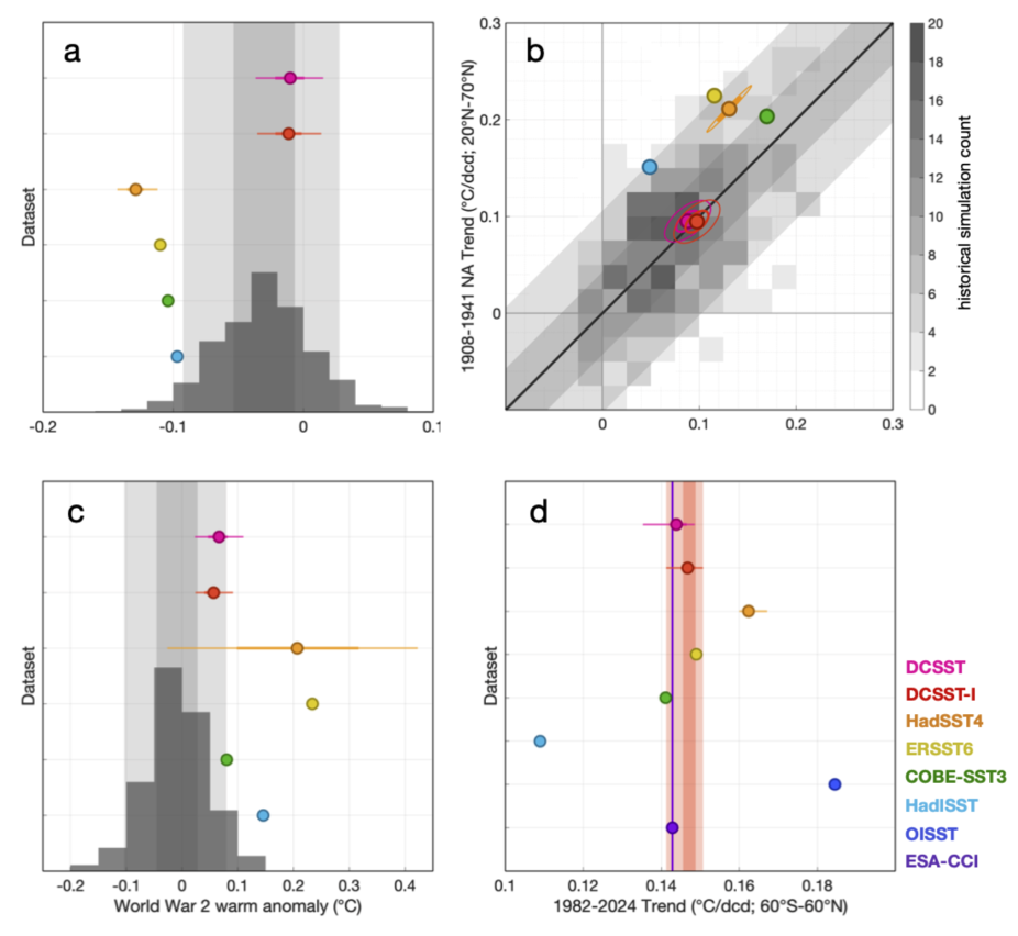
Figure 2. Evaluation of biases in different SST products. (a) Early 20th century cold SST anomaly, calculated as the mean SST difference over 1900-1930 relative to a linear fit using 1890-1889 and 1931-1940 data (following Sippel et al., 2024). Markers denote the mean value of a dataset, while thick and thin lines, respectively, denote the interquartile range and 90% confidence interval (c.i.), where an ensemble is available. The histogram presents the distribution estimated from 550 historical simulations from 57 CMIP6 models (Eyring et al., 2016), and the dark and light shading denotes, respectively, the interquartile and 90% c.i. (5%-95%). (b) North Atlantic (y-axis) versus North Pacific (x-axis) SST trends over 1908-1941 (following Chan et al., 2019). Markers are as (a), and ellipses denote 1 s.d. and 2 s.d. uncertainty using a bivariate Gaussian fit. Heat map represent the histogram of the 550 CMIP6 historical simulations. The black line depicts the one-to-one relationship, and dark and light shadings denotes, respectively, the interquartile range and 90% c.i. of the simulated inter-basin trend difference. (c) as (a) but for World War 2 warm anomaly, calculated as the 60°S-70°N mean SST anomaly over 1941-1945, relative to the mean over 1935-1940 and 1946-1950 (following Chan and Huybers, 2021). (d) as (a) but for 1982-2024 trend of 60°S-60°N mean SST (following Menemenlis et al., 2025). Note that the trend is over 1982-2020 for COBE-SST3 because data is only available until 2020. For comparison purpose, the red shading shows the interquartile range and the 90% c.i. for DCENT-I, and the vertical purple line denotes the trend of ESA-CCI SST3.0.
Figure 2a shows the test for a cold bias in the first part of the 20th century that is related to bucket measurements that are biased particularly cold (Sippel et al. 2024). The only data products that fall within the range of variability shown in the climate models are the two DCSST estimates which apply an adjustment that reconciles coastal variations over the ocean with those over land. In this early 20th century period this adjustment acts to increase the SST to better align the temperatures on each side of the coastal boundary.
The second test (Figure 2b) examines the differences in trends in the North Atlantic and the North Pacific. Different ocean regions are typically sampled by ships of different nations, with national preferences for different measurement methods and protocols. The most dramatic expression of these national differences is in the trends calculated for different ocean basins as in this test. DCSST is the only dataset to apply an explicit adjustment for such inhomogeneities, in this case identifying not only differences in measurement methods but also the impact of past data management practices: the truncation (rather than rounding) of some Japanese SST and air temperature observations when they were transferred to punch cards. This affected trends in the North Pacific where Japanese observations are concentrated.
The third test (Figure 2c) is for the well-known warm bias during World War 2 where the conflict caused rapid changes in the composition of the observing fleet, measurement methods and observing practices. The data products that show consistency with climate model variability at the 90% confidence level are the two DCSST datasets and COBE-SST3, both using coastal land/ocean contrasts to adjust the SST.
The final test examines global (60°S-60°N) trends in SST since 1982 (Figure 2d). For this period the high-quality ESA-CCI dataset can be used as a reference. Two datasets stand out has having anomalous trends in this test. HadISST is an older data product, although still updated and commonly used. The methodology for HadISST predates the change to using modern observations as a reference, so the trends in HadISST are too low because ship observations for the pre-drifting buoy era (in this case 1980s and early 1990s) are biased warm, decreasing the trend. OISST, and to a lesser extent HadSST4, show higher than expected trends.
Satellite derived climate datasets typically take one of two approaches to bias adjustment to quantify and reduce biases including those due to orbital drift, atmospheric aerosols, cloud detection and accounting for the skin to bulk SST differences. The most common approach, as taken by OISSTv2.1 is to adjust for biases in the satellite data using differences from smoothed and filtered in situ observations from ships, buoys and Argo floats. In contrast the SST CCI CDR v3.0 L4 explicitly identifies and adjusts for biases using radiative transfer modelling, inter-source harmonisation and direct estimation of diurnal variations (Embury et al. 2024). This latter approach has the advantage of being almost independent on in situ observations of SST allowing these to be used for evaluation.
How does the data product perform in evaluation and comparisons?
New data products are typically accompanied by evaluations comparing them with other estimates or presenting quality measures. These evaluations help guide product selection, but it is generally good practice to cross check that your conclusions remain robust across different SST datasets.
Figure 2a–c shows one such evaluation, using climate model variability to assess the bias adjustments in the SST component of the DCENT dataset. These tests informed the assessment but were not used for tuning. DCENT outperforms other historical products in these tests, though this may not always hold for others, underscoring the need for multiple evaluation metrics.
Other useful metrics include:
- Performance as lower boundary conditions in atmospheric models.
- Comparison with high quality data subsets, withheld data, or higher quality regional or time limited datasets (as in Figure 2d).
- Internal consistency in spatial and temporal variability.
- Agreement with related parameters such as air temperature, clouds, or pressure derived variability modes.
- Documentation supporting applied adjustments.
Availability of uncertainty estimates
Most of the data products have estimates of uncertainty that aim to capture different contributions to the uncertainty in the gridbox estimates. Each product provides guidance on how to use the uncertainty estimates in calculations such as constructing spatial or temporal averages or trends.
Smoothing and filling of missing grid boxes
For some applications, particularly the running of atmospheric-only climate model simulations, historical SST estimates are needed for the entire ice-free ocean. Thus, some datasets interpolate the available SST over non-sampled regions to obtain global coverage. Some datasets are available as both infilled and non-infilled versions. Note that an infilled version of HadSST4 can be extracted from the HadCRUT5 dataset and DCSST is available as an infilled version via the DCENT-I data product. Each product takes a different approach to constructing the infilled version, most using methods that define the expected relationships between variability at different locations, typically the covariance between anomalies at every point with every other point using a family of methods often referred to as Kriging. The complexity of the spatial relationships varies between products and may be parameterised or directly estimated. Increasingly a range of different approaches, including machine learning techniques are being applied, including to global surface temperature products of which some of the SST data products here form the marine component.
Structural uncertainty
Although each SST product is likely to contain estimates of contributions to uncertainty, these estimates are themselves uncertain. It is therefore important to compare the different data products, and their uncertainty estimates to gain a more complete understanding of the quality of the data. One way of assessing this is the concept of “structural uncertainty” which aim to capture the uncertainty that arises from the choices that are made during the construction of the data product. This can be done within a data product where there is known uncertainty in the assumptions made, typically this approach is used to capture the residual uncertainty due to the bias adjustments using an ensemble. However this approach is limited for an individual data product as some choices are inherent in the method and cannot be changed. This weakness can be remedied to some extent by extending the comparisons to include multiple data products thereby expanding the range of choices included. This comparative approach can be a powerful tool in identifying issues with the data – for example when and where the uncertainty ranges of different data products do not overlap it is clear there is an issue with one or more datasets, or their quantification of uncertainty. Critically there are cases where there are common issues across data products which cannot be identified in this way. It is therefore also important to consider consistency with related information from observations or models. The study of Sippel et al. (2024) made an extensive comparison of global temperatures derived using SST from a wide range of observations and models, with global temperature similarly derived from land-based sources. Such studies are needed to highlight issues across multiple data products arising from biases that have not yet been identified and are an essential contribution to the cycle of data product development, evaluation and improvement.